LAVA Documentation

Computational Aerosciences Branch
NASA Advanced Supercomputing (NAS) Division
Ames Research Center

Joshua L. Anibal, Chase P. Ashby, Michael F. Barad, Francois Cadieux, Christopher J. DeGrendele, Jared C. Duensing, Ercan Dumlupinar, Jeffrey A. Housman, James C. Jensen, James R. Koch, Olivia G. Martin, Abram K. Rodgers, and Emre Sozer

NASA Ames Research Center, Mountain View, California

Alexander W. Aghili, Timothy Chau, David A. Craig Penner, Victor de Carvalho Britto Sousa, Luis dos Santos Fernandes, Brandon Lowe, Nguyen Ly, Kiran Ravikumar, and Gerrit-daniel Stich

Analytical Mechanics Associates, Mountain View, California

Generated on: 06/15/2026
Version: v1.0.1

Overview

Introduction

The Launch, Ascent, and Vehicle Aerodynamics (LAVA) Framework is a suite of Computational Fluid Dynamics (CFD) and multi-physics solvers with accompanying toolsets for pre- and post-processing including grid generation.

With origins in the late 2000's, LAVA has been continually developed in the Computational Aerosciences branch of NASA Ames Research Center to address a wide variety of NASA's fluids modeling and simulation needs. The solver is built on a modern and flexible software architecture with extensive continuous integration testing at scale, pushing the state-of-the-art in both CFD methods and high-performance computing.

LAVA AMS Seminar

Applications

Some notable areas of application have been:

Launch pad pressure and thermal environment analysis, including multi-phase simulations of plume-water interactions, over-pressure wave dynamics, and conjugate heat transfer for launch pad components. These capabilities have been applied to Space Shuttle, Artemis, and commercial launch vehicles.
Aerodynamic performance characterization and sonic boom predictions for the X-59.
Atmospheric re-entry vehicle deceleration simulations, including supersonic parachute deployment with fluid-structure interaction, dynamic stability analysis with 6DOF motion, and supersonic retro-propulsion dynamics.
Aero-acoustic predictions for propulsion systems, including open-rotor noise analysis and X-59 jet noise assessment.
Aerodynamic buffeting mitigation strategies for Artemis at the solid rocket booster forward attachment point.
Conceptual design evaluation and optimization of novel airframe concepts through programs such as SUSAN and HEATHeR.
High-fidelity scale-resolving simulations of aircraft operating with deployed high-lift systems during takeoff and landing phases.

Please see the Applications Gallery for more details on some of these applications.

Solver Capabilities

The development of LAVA's capabilities is guided by the application needs. To enable large-scale simulations with relatively modest compute resources and provide the most efficient and appropriate grid paradigms for each application, LAVA emphasizes both algorithmic innovation and code optimization for high-performance computing environments.

A central philosophy of LAVA is to reduce user-effort and improve error-prone aspects of the CFD workflow through extensive automation and robust tooling. This is exemplified by LAVA's support of multiple meshing paradigms: block-structured curvilinear with overset, Cartesian immersed boundary with Adaptive Mesh Refinement (AMR), and arbitrary polyhedral unstructured meshes. These methods provide users with the flexibility to choose the appropriate mesh paradigm for their specific application, ranging from fully hand-tailored body-fitted curvilinear meshes to partial automation using hybrid curvilinear/immersed-boundary approaches, to fully automated Cartesian or Voronoi unstructured meshes. Additionally, LAVA provides comprehensive in-situ and post-processing tools to streamline the entire simulation workflow.

A high-level overview of LAVA solver capabilities is given below:

Capability	Cartesian	Curvilinear	Unstructured
Mesh type	Cartesian	Block-structured	Arbitrary polyhedral unstructured
Equations	Navier-Stokes	Navier-Stokes	Navier-Stokes
Discretization	Finite difference	Finite difference	Finite volume
Compressibility	Compressible	Compressible	Compressible
Fluid Model	Perfect, Stiffened	Perfect	Perfect
Boundary representation	Immersed Boundary	Body-fitted/immersed boundary	Body-fitted
Mesh transitions	Octree 2:1 interfaces	Overset or multi-block	Conformal
Spatial order of accuracy	2nd, 4th	2nd, 4th	2nd
Temporal order of accuracy (explicit)	2nd, 3rd, 4th	3rd	2nd, 3rd, 4th
Temporal order of accuracy (implicit)	✗	2nd	2nd
Solution Approaches	WMLES	WMLES/HRLES/RANS	WMLES/RANS
Mesh Adaptation	Adaptive mesh refinement	Adjoint based redistribution	✗
Moving bodies	Prescribed/6DOF motion	Prescribed	✗
Multi-species	✓	✗	✓
Multi-phase	✓	✗	✗
Reacting flows	✗	✗	✗
Radiative heat transfer	✗	✗	✗
Fluid-structure interaction	Shell element	✗	✗
Conjugate heat transfer	✗	✗	Coupled 1-D solid conduction
Shape optimization	✗	✓	✗
Hardware	CPU, static geometry on GPU	CPU, WMLES on GPU	CPU, WMLES on GPU

RANS: Reynolds-averaged Navier-Stokes
HRLES: Hybrid Reynolds-averaged Navier-Stokes large-eddy simulation
WMLES: Wall-modeled large-eddy simulation

Gallery

Showcased below is a sampling of application work done with LAVA at NASA. This list is nowhere near exhaustive, but is meant to be illustrative of what LAVA can be used for.

Space

SLS Unsteady Aerodynamics

Simulation of SLS at ascent conditions.

Launch Pad Environment

Simulation of SLS exhaust plume and acoustic suppression system dynamics.

Supersonic Parachute Deployment

Parachute FSI simulation of ASPIRE flight test.

Crew Launch Abort

Orion abort vehicle analysis showing exhaust plume dynamics.

Mars Vehicle Entry

Supersonic retropropulsion simulation of Mars concept vehicle.

Aeronautics

Aerodynamic Shape Optimization

CFD-based refinement of the CRM wing at cruise.

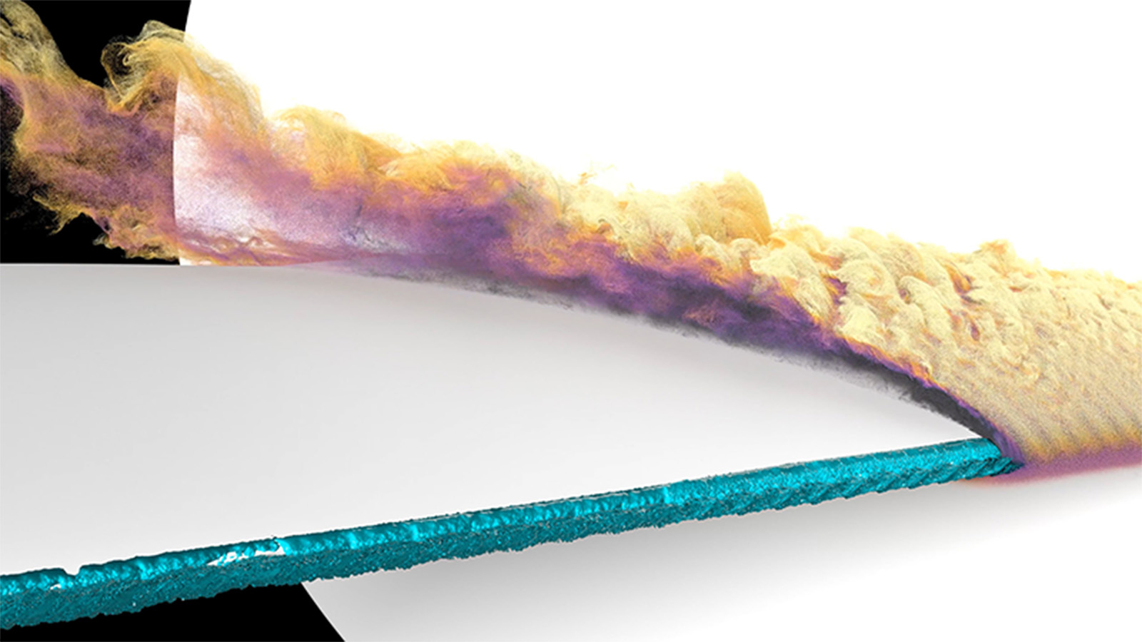
Iced Aerodynamics

Leading-Edge Ice on the CRM Wing modeled with WMLES.

High-Lift Prediction

Simulation of High-Lift for the HLPW.

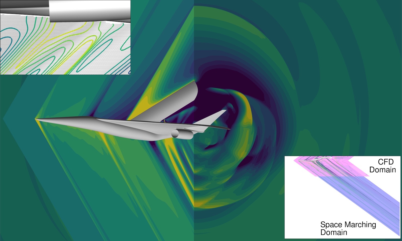
X-59 Boom Prediction

Near field X-59 Supersonic Demonstrator acoustics.

Supersonic Jet Noise

Noise prediction of supersonic jet concepts.

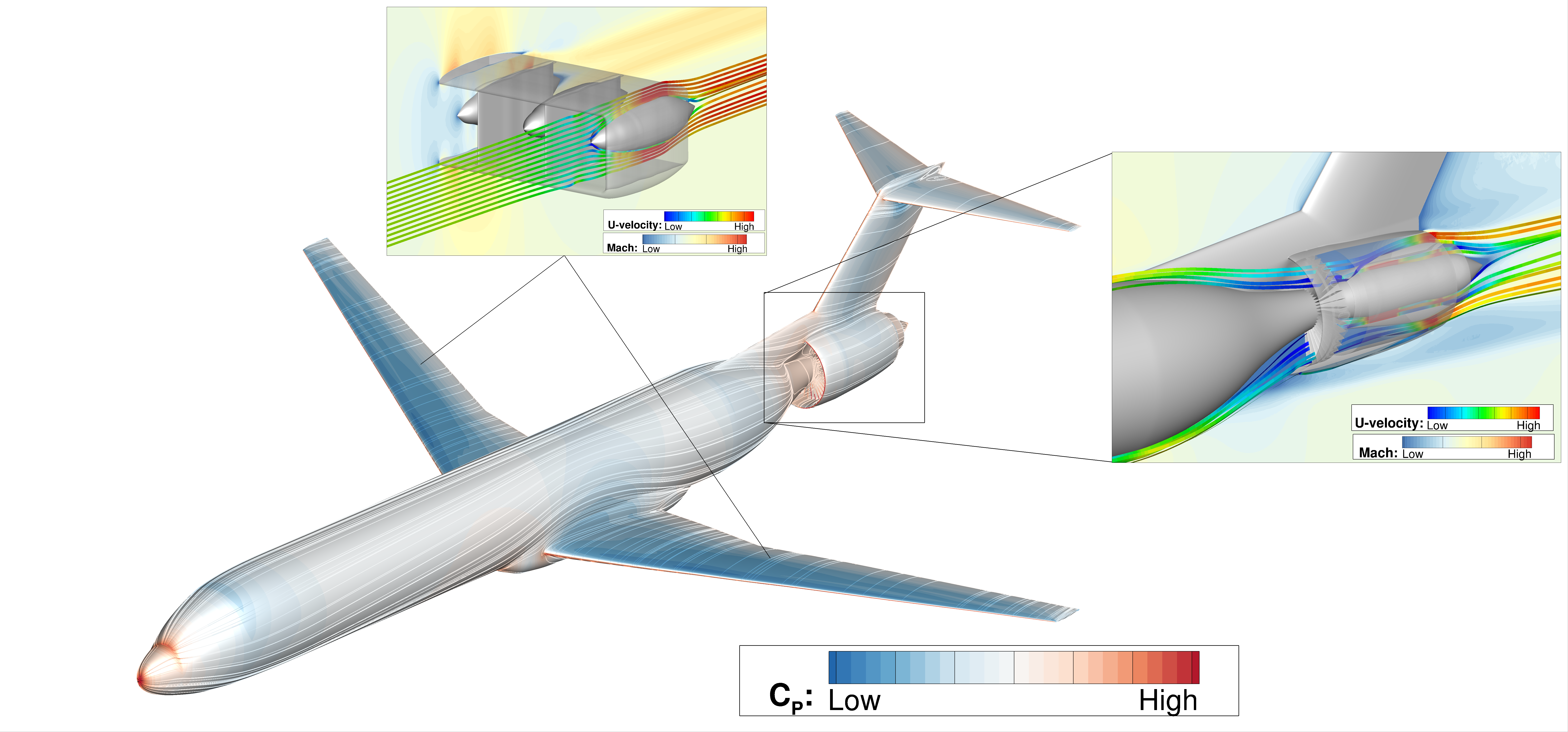
BLI & DEP Assessment

SUSAN concept analysis with distributed electric propulsion and boundary layer ingestion.

TTBW Transonic Buffet

Unsteady shock motion and buffet analysis on TTBW concept.

Open rotor analysis

Acoustic analysis of novel open-rotor designs.

Jet Engine Fan

Fan blade performance assessment.

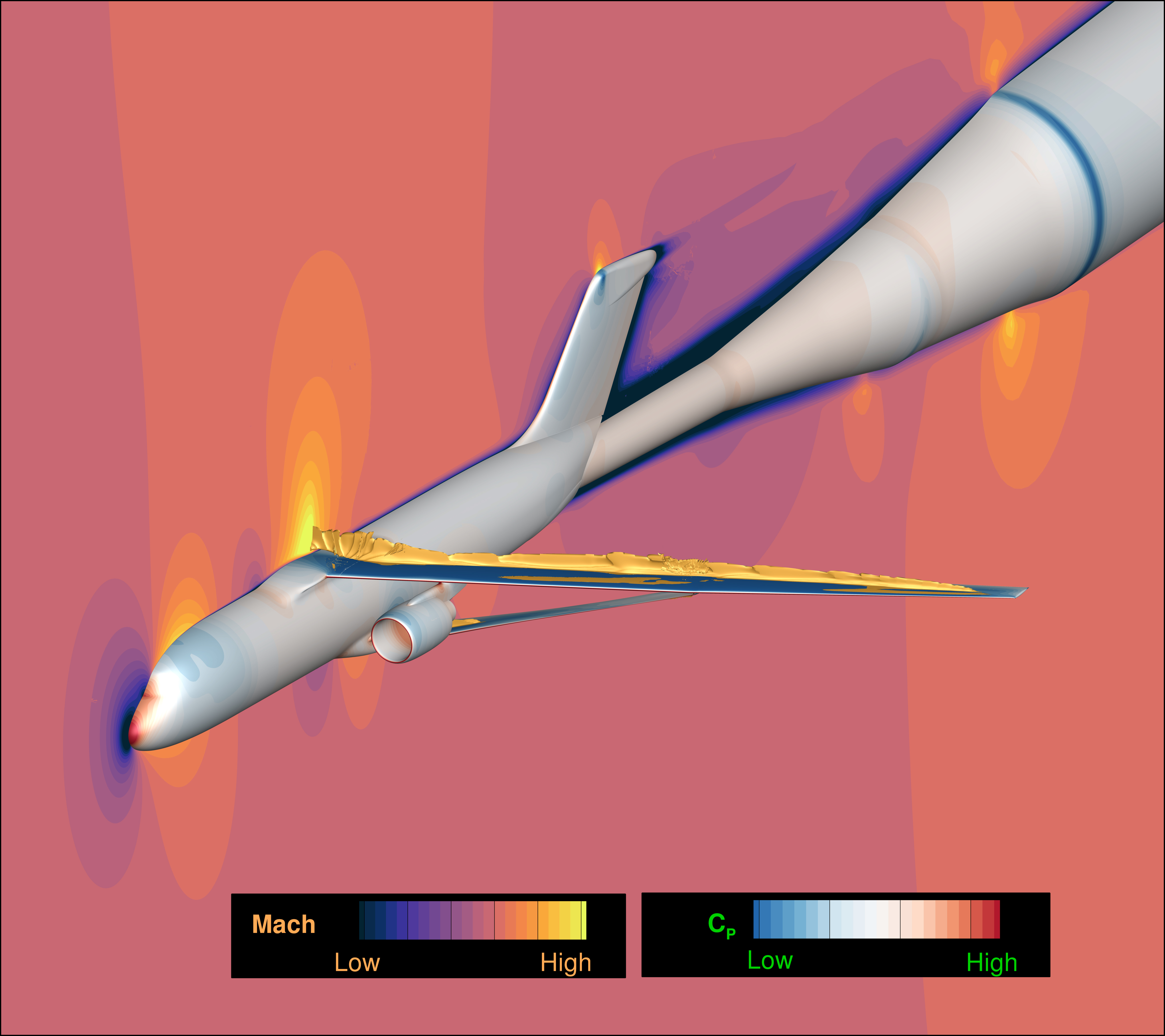
Novel Aircraft Performance

Performance assessment of a transonic truss-braced wing.

Aircraft Stability

Dynamic stability analysis of the X-57 with forced oscillation simulation.

Tutorials Overview

There are download links throughout the tutorials, but you can also download all the tutorial files (except for the meshes) as a tarball.

tutorial_files.tar.gz

Uncompressing the tarball should create a neat file structure organized by <tutorial case>/<solver type>, you can do this with.

tar -xzf tutorial_files.tar.gz

Similarly, to download all the meshes at once and place them in the expanded source tree you can run

wget -r -np -erobots=off -nH --cut-dirs=1 -P tutorial_files/ https://data.nas.nasa.gov/lava/
find tutorial_files/ -name "index.html" -delete

This will download GBs of data and thus may take some time. The second command simply cleans the unwanted index.html files used by wget. You can download the meshes one at a time from the NAS data-portal website or from the links embedded in the tutorials throughout.

Tutorial Map

Below is a map of the tutorials available for each solver.

Version Notes

As new versions of LAVA are released you can find information on the fixes and features added by each version here.

1.0.1

LAVA 1.0.1 is a patch release with bug fixes, input naming cleanup, and general improvements across all three solvers.

Cartesian solver: Bug fixes address time-averaging EMA restart correctness, HWCNS positivity logic, multiphase nozzle and equilibrium input validation, and immersed boundary and AMR robustness. The default convective flux function changes from Rusanov to HLLEC for improved low-Mach accuracy. New features include volume subset output, an overhauled turbulence transition sensor, the wmpartialslip immersed BC, and new IB diagnostic surface output variables.

Unstructured solver: Bug fixes address time-averaging reset correctness, wall-model TKE sensor numerical stability, CFL diagnostic inconsistency, surface output ordering across MPI configurations, and problem cell output with high rank counts. New features include wall-normal line probe output for u⁺/y⁺ post-processing, anisotropic LES Vreman filter size, solution-linked surface CGNS output, compact binary BC statistics, automatic Jacobian epsilon selection, and problem-cell CGNS dumps on abort.

Cartesian and Unstructured: Exponential moving average (EMA) time-averaging inputs are renamed from ...timescale... to ...window.... Old names still accepted with a deprecation warning. A nozzle ASCII radial table validation fix and the new LAVAParaviewPlugin.py for ParaView mask visualization apply to both solvers.

Curvilinear solver: New extrapolation order and type options for viscous and inviscid wall boundary conditions.

Cartesian Solver (CART)

Bug fix: Cart surface time-averaging EMA lost its sample timestamp across restarts, causing an inflated alpha on the first post-restart sample. prevTime is now persisted per surface in the restart file.
Bug fix: Positivity-preserving logic for HWCNS interpolation was not applied uniformly across all state components. The scheme now treats all state components equally.
Bug fix: Multiphase nozzle with asciiLineReadSpecies now requires the largest file mass fraction to match ispecies.
Bug fix: Improved robustness of multiphaseequilibrium functionality for multiphase state input to a wide range of user's state input.
Bug fix: Improved robustness of immersed boundary and adaptive mesh refinement functionality.
Input rename: AMR error-metric EMA inputs renamed: errormetricexponentialmovingaveragetimescalectu → errormetricexponentialmovingaveragewindowctu (and ...timescale → ...window for the physical-time variant). Old names deprecated.
The default convective flux function has changed from Rusanov to HLLEC. HLLEC provides better accuracy for low-Mach-number flows while remaining robust for high-speed and shocked flows. Cases that explicitly set fluxfunction in their input file are unaffected.
Volume subset output: support for writing subsets of the domain (box type) with independent output intervals per subset.
Transition sensor overhaul: improved robustness, OpenMP threading, and restart support for the turbulence transition sensor.
New wmpartialslip immersed BC: applies wall-model-driven slip velocity at immersed wall cells, improving consistency with the convective operator. The transition height between slip and no-slip behavior (partialslipheight, in wall units y⁺) is configurable; the default is y⁺ = 100. Adds a new partialslip surface output variable (0 = no-slip region, 1 = slip region) and suppresses qdot/turbulence surface outputs for BC configurations where they are not applicable.
Removed a partial-slip wall BC variant that was not reliable for bodies with thin geometry (e.g. thin fins or plates). The wmpartialslip BC should be used instead.
New surface output variables NormalIntoFluidX/Y/Z, Component, and BodyVelocityX/Y/Z are available to help diagnose immersed boundary behavior. These can be added to the surface output variable list in the input file.

Unstructured Solver (UNST)

Bug fix: When time averaging is reset mid-run using resetTimeAvg, the sample interval timer was not zeroed, causing the first new sample after the reset to carry an incorrect time weight. This is now corrected.
Bug fix: Wall-model turbulence-transition TKE sensor used a numerically unstable variance formula (E[U²]−E[U]²). Replaced with Welford online variance, eliminating catastrophic cancellation for high mean velocities.
Bug fix: Small cell filtering diagnostic was inconsistent with the CFL calculation, causing unexpectedly small time steps in rare cases.
Bug fix: Surface output (faces and nodes) is now written in a consistent order regardless of how the mesh is distributed across MPI ranks, ensuring identical surface files when rerunning with a different processor count.
Bug fix: Problem cell output on abort or startup failed when the number of MPI ranks exceeded the number of problem cells. This is now handled correctly.
Wall-normal BL probe: line probes now support wall normal = true mode. Output includes wall shear stress, density, and viscosity at the projected foot for u+/y+ post-processing.
LES Vreman subgrid-scale model now uses anisotropic filter size by default.
Reduced conservatism in the CFL calculation, yielding larger time steps.
Surface CGNS output now uses solution linking by default: a single mesh file (Unst.surf.meshLink.cgns) is written once and each solution file links to it, avoiding redundant geometry data. Disable with splitgridandsolution = false in the surface {} output block.
BC statistics output replaced: per-step ASCII bc_stats_NNNNNNN.dat files are replaced by a continuous binary surface/bc_stats.iter file (same format as monitor/unst.data.iter). A surface/bc_name_map.txt mapping file is written once at startup. Mach-driven pressure history is similarly written to surface/mach_driven_pressure_BCN.iter. Both files support seamless restart continuation.
When running with implicit time stepping or RANS simulation with the numerical Jacobian selected, Jacobian epsilon now defaults to automatic selection based on the magnitude of the solution vector entries.
During startup and when the unstructured solver aborts in robustmode, it now dumps out the problem cells to a CGNS file in the volume output directory with the flow solution.
Surface output is now written in deterministic global id order. Split grid and solution for surface output is now false by default.

Cartesian and Unstructured Solvers (CART/UNST)

Bug fix: Nozzle ASCII radial table length must match asciiLineTimeStart / Stop / Skip and numberofradialpoints.
Input rename: Exponential moving average (EMA) time-averaging inputs renamed: exponentialmovingaveragetimescalectu → exponentialmovingaveragewindowctu (physical-time variant: exponentialmovingaveragetimescale → exponentialmovingaveragewindow). Old names still accepted with a deprecation warning.
Added LAVAParaviewPlugin.py (in bin/) with Process Cart Mask and Process Unst Mask filters for extracting individual bit flags from LAVA cell mask arrays in ParaView.

Curvilinear Solver (CURV)

Bug fix: Fixed bug in restart file reading field mapping between variables available in restart file and those required for restart and read into tile. Fixed bug in unsteady simulation restarts using the SAsLM2015 correlation-based turbulence transition model.
Add normal momentum and constant entropy extrapolation options for BCWallInviscid, BCWallViscous, and BCWallViscousIsothermal walls when using a wall model.
Add linear extrapolation option for BCExtrapolate boundaries.
Add extrapolation order options for BCWallInviscid, BCWallViscous, and BCWallViscousIsothermal walls when using a wall model. Maintains backward compatibility with wallModelOrder.

Tools (TOOLS)

Bug fix: Fixed broken symlinks for some mesh utility tools that were pointing to non-existent binaries.

1.0.0 (2026/03/19)

First public release of LAVA

Our Team

LAVA is developed by a team of NASA civil servants and contractors within the Computational Aerosciences Branch at NASA Ames Research Center.

LAVA Leadership

Jared Duensing

LAVA Team Lead

Jeff Housman

Curvilinear Lead

Emre Sozer

Unstructured Lead

Mike Barad

Cartesian Lead

Gerrit-Daniel Stich

Contractor Lead

LAVA Development Team

Alexander Aghili

Josh Anibal

Chase Ashby

Francois Cadieux

Timothy Chau

Chris DeGrendele

Ercan Dumlupinar

Luis Fernandes

James Jensen

James Koch

Brandon Lowe

Nguyen Ly

Olivia Martin

David Craig Penner

Kiran Ravikumar

Bram Rodgers

Victor Sousa

Acknowledgments

The development and continued progress of LAVA has been made possible through the generous funding and support of multiple NASA programs and projects across the agency. We are deeply grateful to the following mission directorates and their associated programs and projects. We are also grateful to the predecessor projects and programs whose early investments laid the foundation for the LAVA framework. Their sustained commitment to computational fluid dynamics research made LAVA possible.

NASA Program Support

ARMD

Aeronautics Research Mission Directorate

Transformational Tools & Technologies TTT High Speed Flight Project HSF Subsonic Vehicle Technologies & Tools SVTT Subsonic Flight Demonstrator SFD Low Boom Flight Demonstrator LBFD Aerosciences Evaluation & Test Capabilities AETC

ESDMD

Exploration Systems Development Mission Directorate

Exploration Ground Systems EGS Human Landing Systems HLS Space Launch System SLS

STMD

Space Technology Mission Directorate

Entry Systems Modeling ESM

SOMD

Space Operations Mission Directorate

Launch Services Program LSP

Computational Resources

We gratefully acknowledge the NASA Advanced Supercomputing (NAS) Division at NASA Ames Research Center for providing the world-class computational resources that make large-scale LAVA simulations possible and facilitate our development. Through the High End Computing Capability (HECC) program, NAS provides access to state-of-the-art supercomputing systems, mass storage, high-speed networking, and expert IT support that are essential to the continued development, testing, and application of LAVA.

Collaborators

We gratefully acknowledge NVIDIA for their continued support of the LAVA framework through close collaboration, technical guidance, and support for GPU-accelerated development. Access to modern GPU architectures, development tools, and performance engineering expertise has been instrumental in advancing LAVA’s capabilities on heterogeneous computing platforms and in enabling efficient porting and optimization of key solver components.

We gratefully acknowledge the following individuals for their ongoing contributions to the development and advancement of the LAVA framework:

DA

David Appelhans

NVIDIA Dev Tech

LE

Lucas Erlandson

NVIDIA Dev Tech

KR

Kyle Rollins

NAS IT Support

TS

Tim Sandstrom

NAS Visualization

IW

Ingo Wald

NVIDIA Ray Tracing

We also thank our early alpha testers and initial users, whose feedback and real-world use have been invaluable in helping shape and mature the initial release of LAVA:

MH

Michael Harris

NASA KSC

BH

Brian Heberling

NASA GRC

KP

Kristopher Pierson

NASA GRC

DD

Derek Dalle

NASA ARC

Former LAVA Software Contributors

Jordan Angel
Christoph Brehm
Jonathan Boustani
Oliver Browne
Aditya Ghate
Ryan Hass
Gaetan Kenway
Cetin Kiris
Daniel Maldonado
Scott Neuhoff
Michael Piotrowski
Kumar Saurabh
Jacob Wagner
Man-Long Wong

We also gratefully acknowledge the many interns, visiting researchers, and other contributors not individually listed here whose work on predecessor versions of LAVA, as well as on components of the current LAVA framework, helped make the public release of LAVA possible.

Legal Disclaimer

Copyright Notice

Launch Ascent And Vehicle Aerodynamics (LAVA)

Notices

LAVA is provided as a research-oriented computational framework without any express or implied warranties. The accuracy, reliability, and applicability of results generated by LAVA—including all solvers, modules, and post-processing tools—depend on the user's modeling choices, input data, and verification efforts.

By using this software, you acknowledge that you are solely responsible for validating results and ensuring their suitability for your intended purpose. NASA, the LAVA development team, and all contributors or distributing parties assume no liability for any outcomes, damages, or losses arising from the use or misuse of this software.

See the related Software Usage Agreement/License for additional disclaimer, waiver and other liability provisions that apply to the software.

This software may only be used, reproduced, and provided to others as permitted under the terms of the agreement under which it was acquired from the U.S. Government. Otherwise, this software may not be redistributed, shared, or transferred to any unauthorized third parties without explicit permission from the appropriate NASA authorities. Neither title to, nor ownership of, the software is hereby transferred. This notice shall remain on all copies of the software.

Disclaimers

THE SOFTWARE AND/OR TECHNICAL DATA ARE PROVIDED "AS IS" WITHOUT ANY WARRANTY OF ANY KIND, EITHER EXPRESSED, IMPLIED, OR STATUTORY, INCLUDING, BUT NOT LIMITED TO, ANY WARRANTY THAT THE SOFTWARE AND/OR TECHNICAL DATA WILL CONFORM TO SPECIFICATIONS, ANY IMPLIED WARRANTIES OF MERCHANTABILITY, FITNESS FOR A PARTICULAR PURPOSE, OR FREEDOM FROM INFRINGEMENT, ANY WARRANTY THAT THE SOFTWARE AND/OR TECHNICAL DATA WILL BE ERROR FREE, OR ANY WARRANTY THAT TECHNICAL DATA, IF PROVIDED, WILL CONFORM TO THE SOFTWARE. IN NO EVENT SHALL THE UNITED STATES GOVERNMENT, OR ITS CONTRACTORS OR SUBCONTRACTORS, BE LIABLE FOR ANY DAMAGES, INCLUDING, BUT NOT LIMITED TO, DIRECT, INDIRECT, SPECIAL OR CONSEQUENTIAL DAMAGES, ARISING OUT OF, RESULTING FROM, OR IN ANY WAY CONNECTED WITH THIS SOFTWARE AND/OR TECHNICAL DATA, WHETHER OR NOT BASED UPON WARRANTY, CONTRACT, TORT, OR OTHERWISE, WHETHER OR NOT INJURY WAS SUSTAINED BY PERSONS OR PROPERTY OR OTHERWISE, AND WHETHER OR NOT LOSS WAS SUSTAINED FROM, OR AROSE OUT OF THE RESULTS OF, OR USE OF, THE SOFTWARE AND/OR TECHNICAL DATA.

THE UNITED STATES GOVERNMENT DISCLAIMS ALL WARRANTIES AND LIABILITIES REGARDING THIRD PARTY COMPUTER SOFTWARE, DATA, OR DOCUMENTATION, IF SAID THIRD PARTY COMPUTER SOFTWARE, DATA, OR DOCUMENTATION IS PRESENT IN THE NASA SOFTWARE AND/OR TECHNICAL DATA, AND DISTRIBUTES IT "AS IS."

RECIPIENT AGREES TO WAIVE ANY AND ALL CLAIMS AGAINST THE UNITED STATES GOVERNMENT AND ITS CONTRACTORS AND SUBCONTRACTORS, AND SHALL INDEMNIFY AND HOLD HARMLESS THE UNITED STATES GOVERNMENT AND ITS CONTRACTORS AND SUBCONTRACTORS FOR ANY LIABILITIES, DEMANDS, DAMAGES, EXPENSES OR LOSSES THAT MAY ARISE FROM RECIPIENT'S USE OF THE SOFTWARE AND/OR TECHNICAL DATA, INCLUDING ANY DAMAGES FROM PRODUCTS BASED ON, OR RESULTING FROM, THE USE THEREOF.

IF RECIPIENT FURTHER RELEASES OR DISTRIBUTES THE NASA SOFTWARE AND/OR TECHNICAL DATA, RECIPIENT AGREES TO OBTAIN THIS IDENTICAL WAIVER OF CLAIMS, INDEMNIFICATION AND HOLD HARMLESS AGREEMENT WITH ANY ENTITIES THAT ARE PROVIDED WITH THE SOFTWARE AND/OR TECHNICAL DATA.

Third-Party Software

LAVA includes the following third-party software components:

1. BVH

Permission is hereby granted, free of charge, to any person obtaining a copy of this software and associated documentation files (the "Software"), to deal in the Software without restriction, including without limitation the rights to use, copy, modify, merge, publish, distribute, sublicense, and/or sell copies of the Software, and to permit persons to whom the Software is furnished to do so, subject to the following conditions:

The above copyright notice and this permission notice shall be included in all copies or substantial portions of the Software.

THE SOFTWARE IS PROVIDED "AS IS", WITHOUT WARRANTY OF ANY KIND, EXPRESS OR IMPLIED, INCLUDING BUT NOT LIMITED TO THE WARRANTIES OF MERCHANTABILITY, FITNESS FOR A PARTICULAR PURPOSE AND NONINFRINGEMENT. IN NO EVENT SHALL THE AUTHORS OR COPYRIGHT HOLDERS BE LIABLE FOR ANY CLAIM, DAMAGES OR OTHER LIABILITY, WHETHER IN AN ACTION OF CONTRACT, TORT OR OTHERWISE, ARISING FROM, OUT OF OR IN CONNECTION WITH THE SOFTWARE OR THE USE OR OTHER DEALINGS IN THE SOFTWARE.

2. kdtree

Redistribution and use in source and binary forms, with or without modification, are permitted provided that the following conditions are met:

Redistributions of source code must retain the above copyright notice, this list of conditions and the following disclaimer.
Redistributions in binary form must reproduce the above copyright notice, this list of conditions and the following disclaimer in the documentation and/or other materials provided with the distribution.
The name of the author may not be used to endorse or promote products derived from this software without specific prior written permission.

THIS SOFTWARE IS PROVIDED BY THE AUTHOR "AS IS" AND ANY EXPRESS OR IMPLIED WARRANTIES, INCLUDING, BUT NOT LIMITED TO, THE IMPLIED WARRANTIES OF MERCHANTABILITY AND FITNESS FOR A PARTICULAR PURPOSE ARE DISCLAIMED. IN NO EVENT SHALL THE AUTHOR BE LIABLE FOR ANY DIRECT, INDIRECT, INCIDENTAL, SPECIAL, EXEMPLARY, OR CONSEQUENTIAL DAMAGES (INCLUDING, BUT NOT LIMITED TO, PROCUREMENT OF SUBSTITUTE GOODS OR SERVICES; LOSS OF USE, DATA, OR PROFITS; OR BUSINESS INTERRUPTION) HOWEVER CAUSED AND ON ANY THEORY OF LIABILITY, WHETHER IN CONTRACT, STRICT LIABILITY, OR TORT (INCLUDING NEGLIGENCE OR OTHERWISE) ARISING IN ANY WAY OUT OF THE USE OF THIS SOFTWARE, EVEN IF ADVISED OF THE POSSIBILITY OF SUCH DAMAGE.

3. libyaml

Permission is hereby granted, free of charge, to any person obtaining a copy of this software and associated documentation files (the "Software"), to deal in the Software without restriction, including without limitation the rights to use, copy, modify, merge, publish, distribute, sublicense, and/or sell copies of the Software, and to permit persons to whom the Software is furnished to do so, subject to the following conditions:

The above copyright notice and this permission notice shall be included in all copies or substantial portions of the Software.

THE SOFTWARE IS PROVIDED "AS IS", WITHOUT WARRANTY OF ANY KIND, EXPRESS OR IMPLIED, INCLUDING BUT NOT LIMITED TO THE WARRANTIES OF MERCHANTABILITY, FITNESS FOR A PARTICULAR PURPOSE AND NONINFRINGEMENT. IN NO EVENT SHALL THE AUTHORS OR COPYRIGHT HOLDERS BE LIABLE FOR ANY CLAIM, DAMAGES OR OTHER LIABILITY, WHETHER IN AN ACTION OF CONTRACT, TORT OR OTHERWISE, ARISING FROM, OUT OF OR IN CONNECTION WITH THE SOFTWARE OR THE USE OR OTHER DEALINGS IN THE SOFTWARE.

4. Geogram

Redistribution and use in source and binary forms, with or without modification, are permitted provided that the following conditions are met:

Redistributions of source code must retain the above copyright notice, this list of conditions and the following disclaimer.
Redistributions in binary form must reproduce the above copyright notice, this list of conditions and the following disclaimer in the documentation and/or other materials provided with the distribution.
Neither the name of Inria nor the names of its contributors may be used to endorse or promote products derived from this software without specific prior written permission.

THIS SOFTWARE IS PROVIDED BY THE COPYRIGHT HOLDERS AND CONTRIBUTORS "AS IS" AND ANY EXPRESS OR IMPLIED WARRANTIES, INCLUDING, BUT NOT LIMITED TO, THE IMPLIED WARRANTIES OF MERCHANTABILITY AND FITNESS FOR A PARTICULAR PURPOSE ARE DISCLAIMED. IN NO EVENT SHALL THE COPYRIGHT HOLDER OR CONTRIBUTORS BE LIABLE FOR ANY DIRECT, INDIRECT, INCIDENTAL, SPECIAL, EXEMPLARY, OR CONSEQUENTIAL DAMAGES (INCLUDING, BUT NOT LIMITED TO, PROCUREMENT OF SUBSTITUTE GOODS OR SERVICES; LOSS OF USE, DATA, OR PROFITS; OR BUSINESS INTERRUPTION) HOWEVER CAUSED AND ON ANY THEORY OF LIABILITY, WHETHER IN CONTRACT, STRICT LIABILITY, OR TORT (INCLUDING NEGLIGENCE OR OTHERWISE) ARISING IN ANY WAY OUT OF THE USE OF THIS SOFTWARE, EVEN IF ADVISED OF THE POSSIBILITY OF SUCH DAMAGE.

5. yaml-cpp

Permission is hereby granted, free of charge, to any person obtaining a copy of this software and associated documentation files (the "Software"), to deal in the Software without restriction, including without limitation the rights to use, copy, modify, merge, publish, distribute, sublicense, and/or sell copies of the Software, and to permit persons to whom the Software is furnished to do so, subject to the following conditions:

The above copyright notice and this permission notice shall be included in all copies or substantial portions of the Software.

THE SOFTWARE IS PROVIDED "AS IS", WITHOUT WARRANTY OF ANY KIND, EXPRESS OR IMPLIED, INCLUDING BUT NOT LIMITED TO THE WARRANTIES OF MERCHANTABILITY, FITNESS FOR A PARTICULAR PURPOSE AND NONINFRINGEMENT. IN NO EVENT SHALL THE AUTHORS OR COPYRIGHT HOLDERS BE LIABLE FOR ANY CLAIM, DAMAGES OR OTHER LIABILITY, WHETHER IN AN ACTION OF CONTRACT, TORT OR OTHERWISE, ARISING FROM, OUT OF OR IN CONNECTION WITH THE SOFTWARE OR THE USE OR OTHER DEALINGS IN THE SOFTWARE.

6. Pyoptsparse

LAVA uses Pyoptsparse, a third-party library licensed under LGPL License 3.0.

For the complete text of the GNU Lesser General Public License v3.0 and GNU General Public License v3.0, please visit: - LGPL v3: https://www.gnu.org/licenses/lgpl-3.0.html - GPL v3: https://www.gnu.org/licenses/gpl-3.0.html

7. Intel MKL

The LAVA executables compiled with Intel compilers statically link MKL which is distributed under the Intel Simplified Software License (Version October 2022)

PIN: Copyright (C) Intel Corporation

Use and Redistribution. You may use and redistribute the software, which is provided in binary form only, (the "Software"), without modification, provided the following conditions are met:

Redistributions must reproduce the above copyright notice and these terms of use in the Software and in the documentation and/or other materials provided with the distribution.
Neither the name of Intel nor the names of its suppliers may be used to endorse or promote products derived from this Software without specific prior written permission.
No reverse engineering, decompilation, or disassembly of the Software is permitted, nor any modification or alteration of the Software or its operation at any time, including during execution.

No other licenses. Except as provided in the preceding section, Intel grants no licenses or other rights by implication, estoppel or otherwise to, patent, copyright, trademark, trade name, service mark or other intellectual property licenses or rights of Intel.

Third party software. "Third Party Software" means the files (if any) listed in the "third-party-software.txt" or other similarly-named text file that may be included with the Software. Third Party Software, even if included with the distribution of the Software, may be governed by separate license terms, including without limitation, third party license terms, open source software notices and terms, and/or other Intel software license terms. These separate license terms solely govern Your use of the Third Party Software.

DISCLAIMER. THIS SOFTWARE IS PROVIDED "AS IS" AND ANY EXPRESS OR IMPLIED WARRANTIES, INCLUDING, BUT NOT LIMITED TO, THE IMPLIED WARRANTIES OF MERCHANTABILITY, FITNESS FOR A PARTICULAR PURPOSE, AND NON-INFRINGEMENT ARE DISCLAIMED. THIS SOFTWARE IS NOT INTENDED FOR USE IN SYSTEMS OR APPLICATIONS WHERE FAILURE OF THE SOFTWARE MAY CAUSE PERSONAL INJURY OR DEATH AND YOU AGREE THAT YOU ARE FULLY RESPONSIBLE FOR ANY CLAIMS, COSTS, DAMAGES, EXPENSES, AND ATTORNEYS' FEES ARISING OUT OF ANY SUCH USE, EVEN IF ANY CLAIM ALLEGES THAT INTEL WAS NEGLIGENT REGARDING THE DESIGN OR MANUFACTURE OF THE SOFTWARE.

LIMITATION OF LIABILITY. IN NO EVENT WILL INTEL BE LIABLE FOR ANY DIRECT, INDIRECT, INCIDENTAL, SPECIAL, EXEMPLARY, OR CONSEQUENTIAL DAMAGES (INCLUDING, BUT NOT LIMITED TO, PROCUREMENT OF SUBSTITUTE GOODS OR SERVICES; LOSS OF USE, DATA, OR PROFITS; OR BUSINESS INTERRUPTION) HOWEVER CAUSED AND ON ANY THEORY OF LIABILITY, WHETHER IN CONTRACT, STRICT LIABILITY, OR TORT (INCLUDING NEGLIGENCE OR OTHERWISE) ARISING IN ANY WAY OUT OF THE USE OF THIS SOFTWARE, EVEN IF ADVISED OF THE POSSIBILITY OF SUCH DAMAGE.

No support. Intel may make changes to the Software, at any time without notice, and is not obligated to support, update or provide training for the Software.

Termination. Your right to use the Software is terminated in the event of your breach of this license.

Feedback. Should you provide Intel with comments, modifications, corrections, enhancements or other input ("Feedback") related to the Software, Intel will be free to use, disclose, reproduce, license or otherwise distribute or exploit the Feedback in its sole discretion without any obligations or restrictions of any kind, including without limitation, intellectual property rights or licensing obligations.

Compliance with laws. You agree to comply with all relevant laws and regulations governing your use, transfer, import or export (or prohibition thereof) of the Software.

Governing law. All disputes will be governed by the laws of the United States of America and the State of Delaware without reference to conflict of law principles and subject to the exclusive jurisdiction of the state or federal courts sitting in the State of Delaware, and each party agrees that it submits to the personal jurisdiction and venue of those courts and waives any objections. THE UNITED NATIONS CONVENTION ON CONTRACTS FOR THE INTERNATIONAL SALE OF GOODS (1980) IS SPECIFICALLY EXCLUDED AND WILL NOT APPLY TO THE SOFTWARE.

8. Intel runtime libraries

The LAVA executables compiled with Intel compilers statically link the Intel runtime libraries - Intel® Fortran Core Library (libifcoremt) - Intel® Math Library (libimf) - Intel® OpenMP Runtime Library (libiomp5) - Intel® Runtime Core Library (libirc) - Intel® Random Number Generator Library (libirng) - Intel® Short Vector Math Library (libsvml)

These libraries are provided by Intel Corporation under the "Intel End User License Agreement for Developer Tools." Redistribution and use in binary form, without modification, are permitted provided that the following conditions are met:

Redistributions in binary form must reproduce the above copyright notice, this list of conditions, and the following disclaimer in the documentation and/or other materials provided with the distribution.
No reverse engineering, decompilation, or disassembly of these libraries is permitted.
Neither the name of Intel Corporation nor the names of its suppliers may be used to endorse or promote products derived from this software without specific prior written permission.

DISCLAIMER: THIS SOFTWARE IS PROVIDED BY INTEL "AS IS" AND ANY EXPRESS OR IMPLIED WARRANTIES, INCLUDING, BUT NOT LIMITED TO, THE IMPLIED WARRANTIES OF MERCHANTABILITY AND FITNESS FOR A PARTICULAR PURPOSE ARE DISCLAIMED. IN NO EVENT SHALL INTEL BE LIABLE FOR ANY DIRECT, INDIRECT, INCIDENTAL, SPECIAL, EXEMPLARY, OR CONSEQUENTIAL DAMAGES (INCLUDING, BUT NOT LIMITED TO, PROCUREMENT OF SUBSTITUTE GOODS OR SERVICES; LOSS OF USE, DATA, OR PROFITS; OR BUSINESS INTERRUPTION) HOWEVER CAUSED AND ON ANY THEORY OF LIABILITY, WHETHER IN CONTRACT, STRICT LIABILITY, OR TORT (INCLUDING NEGLIGENCE OR OTHERWISE) ARISING IN ANY WAY OUT OF THE USE OF THIS SOFTWARE, EVEN IF ADVISED OF THE POSSIBILITY OF SUCH DAMAGE.

Setup and Utilities

LAVA Access Guide

LAVA is released through the NASA Software Catalog.

LAVA

NAS Users (Module-Based Access): If you have access to NASA Advanced Supercomputing (NAS) systems and want to run LAVA there, use the module system.
External Users (Tarball Installation): If you would like to run LAVA on your own system, AWS or other cloud services, download pre-compiled binaries and install LAVA locally.

LAVA Voronoi

LAVA Voronoi is a specialized mesh generation tool that creates polyhedral-cell tessellations for two- and three-dimensional computational domains. It is released along with LAVA through the NASA Software Catalog.

NAS Users (Module-Based Access): If you have access to NASA Advanced Supercomputing (NAS) systems and want to run LAVA there, use the module system.
External Users (Tarball Installation): If you would like to run Voronoi mesher on your own system, AWS or other cloud services, download pre-compiled binaries and install locally.

Executables

LAVA: See the full list of supported executables here.
LAVA Voronoi: lavavoro.AVX2 (hybrid MPI+OpenMP, AVX2-optimized for x86_64 CPUs).

LAVA on NAS

See LAVA on NAS for platform-specific notes and recommendations.

Getting Help

Documentation: LAVA Documentation
Contact and LAVA User Community: Contact Us
NAS System Support: For NAS-specific issues, contact NAS User Services

LAVA Access for NAS Users

If you have access to NASA Advanced Supercomputing (NAS) systems with compute time allocations, a valid Software User Agreement, and want to run LAVA on NAS, submit a NAMS request on IdMax (Launch, Ascent, and Vehicle Aerodynamics (LAVA) Computational Fluid Dynamics (CFD) Access on NAS). Once approved, you can use the module system described below.

Please note the LAVA development team does not have the authority to grant access or issue computer time on NAS systems. You may visit the following page for instructions on how to request NAS computer resources and to see if you qualify.

If you are an external user, go to External Users (Tarball Installation).

Setup Instructions

Add the LAVA module path:
```
module use /swbuild/LAVA/LAVA_modules
```
Warning

If you use --append in the above command, you might not end up loading the right module below. Please make sure to prepend or use the above command as is to avoid conflicts with other modules.
View available LAVA versions:
```
module avail LAVA
```
Load the LAVA module:
```
module load LAVA
```
Tip

The above will give you access to the latest version of LAVA release. You can also choose to load a specific version of LAVA using module load LAVA/<version>
Start using LAVA:

The module automatically:
- Detects your current system (Aitken, Electra, Athena, Cabeus A100, Cabeus Grace Hopper etc.)
- Loads the appropriate compiler and MPI environment
- Adds the correct LAVA executables to your PATH
- Sets necessary environment variables

Sample PBS scripts to run on NAS

For example PBS scripts and NAS runtime guidance, see Running LAVA on NAS.

Troubleshooting

Module LAVA not found

Solution: Ensure you've added the module path: module use /swbuild/LAVA/LAVA_modules

Wrong architecture executable selected

Solution: The module should auto-detect your system. If issues persist, contact LAVA support.

Module conflicts when loading LAVA on Athena (e.g., PrgEnv-intel conflicts with PrgEnv-cray)

Solution: Run module purge to clear all loaded modules, then load LAVA again:

module purge
module use /swbuild/LAVA/LAVA_modules
module load LAVA/<version>

Permission denied errors when loading LAVA_deps (e.g., ERROR: Permission denied on '/nasa/modulefiles/toss4/cmake')

Loading LAVA_deps/rome_old
  Module ERROR: no such variable
        (read trace on "::env(LAVA_REPO_DIR)")
        invoked from within
    "set base        $::env(LAVA_REPO_DIR)"
        (file "/swbuild/LAVA/LAVA_GROUP/LAVA_modules/LAVA_deps/rome_old" line 14)
    Please contact <root@localhost>

Loading LAVA_voro/dev
  ERROR: Load of requirement 'LAVA_deps' failed
No Modulefiles Currently Loaded.

Solution: This occurs when you have conflicting module paths in your environment (e.g., from /swbuild/LAVA/LAVA_GROUP/LAVA_modules/). Ensure that you are prepending the recommended path:

module purge
module use /swbuild/LAVA/LAVA_modules
module load LAVA/<version>

or use the --prepend option on newer TCL module version systems.

module purge
module use --prepend /swbuild/LAVA/LAVA_modules
module load LAVA/<version>

Make sure to also check your .bashrc or .profile and remove (or comment) other conflicting module paths like module use -a /swbuild/LAVA/LAVA_GROUP/LAVA_modules.

Module loading errors on Athena

Loading PrgEnv-intel/8.6.0
  ERROR: Module cannot be loaded due to a conflict.
    HINT: Might try "module unload PrgEnv-cray" first.

Loading LAVA_deps/intel
  ERROR: Load of requirement PrgEnv-intel failed

Solution: On Athena systems, the global profile script /usr/local/lib/init/global.profile can cause conflicts with LAVA modules. Add this safeguard to your .bashrc or .profile to prevent loading it on Athena:

if [[ $(hostname) != athfe* ]] && [[ $(hostname) != x100* ]] && [ -e /usr/local/lib/init/global.profile ]; then
    . /usr/local/lib/init/global.profile
fi

This ensures the global profile is only sourced on non-Athena systems. Alternatively, the issue might be related to using an incorrect version of the module command. Your scripts might need to be modified to use the correct module command for Athena:

if [ -f /opt/cray/pe/modules/default/init/bash ]; then
  source /opt/cray/pe/modules/default/init/bash
else
  source /usr/local/lib/global.profile
fi

After updating your .bashrc or .profile, start a new terminal session, then try loading the module again. Refer to the following for more details.

Executable not found or module loading errors in PBS jobs on Athena

mbind.x: execvp: lavaunst.3D.NS1.AVX512: No such file or directory
x1000c0s4b0n1.hsn.ath.nas.nasa.gov: rank 0 exited with code 255

or

Loading craype/2.7.35
  ERROR: Conflicting PrgEnv-intel/8.6.0 is loading

Loading PrgEnv-intel/8.6.0
  ERROR: Requirement craype is not loaded

Solution: When running PBS jobs on Athena, the environment may not be properly initialized. Add source ~/.bashrc at the beginning of your PBS script after the PBS directives and before loading LAVA modules:

#!/bin/bash
#PBS -S /bin/bash
#PBS -N lava_turin_job
#PBS -q normal
#PBS -l select=16:ncpus=512:mpiprocs=4:model=tur_ath
#PBS -l walltime=04:00:00
#PBS -j oe
#PBS -r n

# Source your bashrc to initialize the environment properly
source ~/.bashrc

# Load LAVA module
module use /swbuild/LAVA/LAVA_modules
module load LAVA/v1.0.0

# ... rest of your script

This ensures your .bashrc settings (including the Athena-specific global profile exclusion) are applied in the PBS job environment. See the NAS Athena documentation for more details.

Module loading fails due to NFS group limitations (Error: "Permission denied" or modules not loading)

Solution: If you are a member of many Unix groups (more than 16), you may encounter NFS filesystem limitations where only the first 16 groups are loaded, potentially causing access issues to LAVA modules and dependencies.

Symptoms:

Module loading works on some systems but not others
Inconsistent behavior across different frontends
Permission denied errors when accessing module files

Workaround: Use the newgrp command to ensure you're logged into the correct group before loading LAVA:

newgrp <your_group>  # e.g., newgrp n1546
module use /swbuild/LAVA/LAVA_modules
module load LAVA/<version>

You can check which groups you're a member of with groups or id -Gn. Contact your system administrator if you need help determining the correct group to use.

md5sum error when running LAVA executables (Error: md5.c line 18: cannot open file)

ERROR: md5.c line 18: cannot open file: /path/to/lavaunst.3D.NS1.AVX2

Solution: This error is benign and can be safely ignored. NAS systems automatically attempt to compute md5 checksums of all executables for auditing. LAVA binaries are distributed with execute-only permissions, which prevents the md5sum utility from reading the binary file. This does not affect LAVA's functionality - the executable will run correctly despite this error message appearing in your output.

Cannot find executable mbind.x

Cannot find executable mbind.x

Solution: The module should add the path to mbind to your environment. But for any reason if you see an error similar to the above use the full path in your run command or PBS script:

All systems except GH:
```
/u/scicon/tools/bin/mbind.x
```
GH systems:
```
/u/scicon/tools/arm/bin/mbind.x
```

LAVA Access validation failed

[I]   Using access file: /path/to/access/file
[E]  (Rank=00000) LAVA Access validation failed.
 Reason: User '<userid>' not authorized for this license

Solution: This is very unlikely and should not happen when you are loading the LAVA release modules. But if it does you can try unset LAVA_ACCESS_FILE.

LAVA Installation for External Users

If you do not have NAS system access, install LAVA using the pre-compiled tarballs from the NASA Software Catalog.

If you are a NAS user, go to NAS Users (Module-Based Access).

Acquiring LAVA

Download the appropriate tarball for your system from the NASA Software Catalog. Tarballs are named using the following convention:

LAVA_<version>_<compiler>_<mpi>_<arch>_<DateStamp>.tar.gz

Example: LAVA_v1.0.0_NVIDIA_OpenMPI_x86_64_2026.03.02.tar.gz

Version numbers follow the format [MAJOR].[MINOR].[PATCH].

Available Build Configurations

LAVA provides four pre-built configurations optimized for different hardware platforms:

Tarball Name	Compiler	MPI	Architecture	Target Systems
`LAVA__NVIDIA_OpenMPI_x86_64_.tar.gz`	NVHPC 25.3	OpenMPI 4.1.6	x86_64 (AVX2)	NVIDIA A100 GPUs, RTX 5090, RTX 4090
`LAVA__NVIDIA_HPCX_aarch64_.tar.gz`	NVHPC 25.3	HPC-X	aarch64 (ARM)	NVIDIA GH200 (Grace-Hopper)
`LAVA__Intel_OpenMPI_x86_64_.tar.gz`	Intel 2023.2.1	OpenMPI 4.1.5	x86_64 (AVX2 & AVX512)	Intel/AMD CPUs (Haswell, Skylake, Rome, Milan, Genoa)
`LAVA__Intel_Cray-MPICH_x86_64_.tar.gz`	Intel 2023.2.1	Cray-MPICH	x86_64 (AVX512)	AMD Turin (Zen 5)

Note

Companies in tarball names above were not involved in generating the LAVA binaries. They only convey compiler information.

Tip

While the Intel and Nvidia binaries were compiled with compiler versions that are older than the most recent available compilers, at runtime the user can choose to use the latest Intel or Nvidia runtime and the binaries should be compatible.

Which Tarball to Download

GPU Systems

Your Hardware	Minimum Compute Capability Supported	Recommended Tarball
NVIDIA A100, RTX 5090, RTX 4090 (x86_64 systems)	SM 8.0+	`LAVA__NVIDIA_OpenMPI_x86_64_.tar.gz`
NVIDIA GH200 (Grace-Hopper ARM systems)	SM 9.0+	`LAVA__NVHPC_HPCX_aarch64_.tar.gz`

CPU-Only Systems (Intel/AMD)

Your CPU	Instruction Set Support	Recommended Tarball
Intel Haswell, Broadwell, Skylake (non-X) AMD Zen, Zen 2, Zen 3, Zen 4 (Rome, Milan, Genoa)	AVX2	`LAVA__Intel_OpenMPI_x86_64_.tar.gz` (use AVX2 executables)
Intel Skylake-X, Cascade Lake, Ice Lake, Sapphire Rapids AMD Zen 5 (Turin)	AVX512	`LAVA__Intel_OpenMPI_x86_64_.tar.gz` (use AVX512 executables) or `LAVA__Intel_Cray-MPICH_x86_64_.tar.gz`

Note

The Intel_OpenMPI_x86_64 tarball includes both AVX2 and AVX512 executables with double and single precision variants. Use AVX2 versions for broader compatibility if unsure of your CPU capabilities.

Note

LAVA and its tools require CPUs with AVX2 instruction set at a minimum.

Installation Steps

Extract the tarball

tar -xzf LAVA_<version>_<compiler>_<mpi>_<arch>_<DateStamp>.tar.gz
cd LAVA_<version>_<compiler>_<mpi>_<arch>

The extracted directory contains:

bin/ - All LAVA executables and utility scripts
lib/ - Curvilinear libraries and Python packages (Intel builds only)
species/ - Species database files

Set up your environment

Load the required modules and set environment variables like LD_LIBRARY_PATH based on your configuration.

Environment Setup for NVIDIA + OpenMPI (x86_64 GPU Systems)

Tarball: LAVA_*_NVIDIA_OpenMPI_x86_64_*.tar.gz

Required Software

OpenMPI 4.1.6 or later
NVIDIA GPU driver version 570.26 or later (required for CUDA 12.8 support)
See NVIDIA CUDA-Driver Compatibility for driver requirements
NVIDIA runtime libraries (any version compatible with CUDA 12.8+)

Note

This tarball was compiled with NVHPC 25.3, but you can use newer NVHPC versions (e.g., 25.11 or later) at runtime. The NVHPC runtime libraries are backward compatible.

Environment Setup:

# If using modules (recommended)
module load nvhpc/25.11
module load openmpi/4.1.6

# Set LAVA necessary env variables
export LAVA_INSTALL_DIR=/path/to/LAVA/install
export LAVA_OUTPUT_INTERVAL=1000000

# Add LAVA binaries to PATH
export PATH=/path/to/LAVA/bin:${PATH}

# If NOT using modules, manually set LD_LIBRARY_PATH
# The following paths are required (adjust versions/paths for your installation):
export LD_LIBRARY_PATH=\
/path/to/nvhpc/compilers/lib:\
/path/to/nvhpc/cuda/lib64:\
/path/to/openmpi/lib:\
${LD_LIBRARY_PATH}

# Example for a typical NVHPC 25.3 installation:
# export LD_LIBRARY_PATH=\
# /opt/nvidia/hpc_sdk/Linux_x86_64/25.3/compilers/lib:\
# /opt/nvidia/hpc_sdk/Linux_x86_64/25.3/cuda/lib64:\
# /opt/openmpi/4.1.6/lib:\
# ${LD_LIBRARY_PATH}

Required Runtime Libraries

The LAVA executable depends on the following dynamic libraries:

NVHPC Compiler Libraries: libcudafor.so, libcudafor_120.so, libnvf.so, libaccdevice.so, libacchost.so, libaccdevaux.so, libnvomp.so, libnvhpcatm.so, libnvc.so, libnvcpumath-avx2.so, libcudadevice.so, libcudanvhpc.so
CUDA Runtime: libcudart.so.12
OpenMPI Libraries: libmpi.so.40, libmpi_mpifh.so.40, libmpi_usempif08.so.40, libmpi_usempi_ignore_tkr.so.40
System Libraries: libz.so.1, librt.so.1, libdl.so.2, libstdc++.so.6, libpthread.so.0, libc.so.6, ld-linux-x86-64.so.2, libgcc_s.so.1, libm.so.6

Verifying Your Setup:

# Check if all dependencies are resolved
ldd /path/to/LAVA/bin/lavacart.3D.NS1

# All libraries should show resolved paths (no "not found")
# If you see "not found", ensure the corresponding library path is in LD_LIBRARY_PATH

Environment Setup for NVIDIA + HPC-X (aarch64 GPU Systems)

Tarball: LAVA_*_NVIDIA_HPCX_aarch64_*.tar.gz

Required Software

HPC-X MPI (bundled with NVHPC or standalone)
NVIDIA GPU driver version 570.26 or later (required for CUDA 12.8 support)
See NVIDIA CUDA-Driver Compatibility for driver requirements
NVHPC runtime libraries (any version compatible with CUDA 12.8+)

Note

This tarball was compiled with NVHPC 25.3, but you can use newer NVHPC versions (e.g., 25.11 or later) at runtime. The NVHPC runtime libraries are backward compatible.

Environment Setup:

# If using modules (recommended)
module load nvhpc-hpcx-cuda12/25.7

# Set LAVA necessary env variables
export LAVA_INSTALL_DIR=/path/to/LAVA/install
export LAVA_OUTPUT_INTERVAL=1000000

# Add LAVA binaries to PATH
export PATH=/path/to/LAVA/bin:${PATH}

# If NOT using modules, manually set LD_LIBRARY_PATH
# The following paths are required (adjust versions/paths for your installation):
export LD_LIBRARY_PATH=\
/path/to/nvhpc/compilers/lib:\
/path/to/nvhpc/cuda/lib64:\
/path/to/nvhpc/comm_libs/12.8/hpcx/hpcx-2.22.1/ompi/lib:\
${LD_LIBRARY_PATH}

# Example for a typical NVHPC 25.3 ARM installation:
# export LD_LIBRARY_PATH=\
# /opt/nvidia/hpc_sdk/Linux_aarch64/25.3/compilers/lib:\
# /opt/nvidia/hpc_sdk/Linux_aarch64/25.3/cuda/lib64:\
# /opt/nvidia/hpc_sdk/Linux_aarch64/25.3/comm_libs/12.8/hpcx/hpcx-2.22.1/ompi/lib:\
# ${LD_LIBRARY_PATH}

Required Runtime Libraries

The LAVA executable depends on the following dynamic libraries:

NVHPC Compiler Libraries: libcudafor.so, libcudafor_120.so, libnvf.so, libaccdevice.so, libacchost.so, libaccdevaux.so, libnvomp.so, libnvhpcatm.so, libnvc.so, libnvcpumath-armv8.so, libnvmalloc.so, libcudadevice.so, libcudanvhpc.so
CUDA Runtime: libcudart.so.12
HPC-X MPI Libraries: libmpi.so.40, libmpi_mpifh.so.40, libmpi_usempif08.so.40, libmpi_usempi_ignore_tkr.so.40
System Libraries: Standard Linux libraries (typically in /usr/lib64 or /lib64)

Verifying Your Setup:

# Check if all dependencies are resolved
ldd /path/to/LAVA/bin/lavacart.3D.NS1

# All libraries should show resolved paths (no "not found")
# If you see "not found", ensure the corresponding library path is in LD_LIBRARY_PATH

Environment Setup for Intel + OpenMPI (CPU Systems)

Tarball: LAVA_*_Intel_OpenMPI_x86_64_*.tar.gz

Required Software

OpenMPI 4.1.5 or later

Environment Setup:

# If using modules (recommended)
module load intel/2022.1.0
module load openmpi/4.1.5

# Set LAVA necessary env variables
export LAVA_INSTALL_DIR=/path/to/LAVA/install
export LAVA_OUTPUT_INTERVAL=1000000

# Add LAVA binaries to PATH
export PATH=/path/to/LAVA/bin:${PATH}

# If NOT using modules, manually set LD_LIBRARY_PATH
# The following paths are required (adjust versions/paths for your installation):
export LD_LIBRARY_PATH=\
/path/to/openmpi/lib:\
${LD_LIBRARY_PATH}

# Example for a typical OpenMPI 4.1.5 installation:
# export LD_LIBRARY_PATH=\
# /opt/openmpi/4.1.5/lib:\
# ${LD_LIBRARY_PATH}

Required Runtime Libraries

The LAVA executable depends on the following dynamic libraries:

OpenMPI Libraries: libmpi.so.40, libmpi_usempif08.so.40, libmpi_usempi_ignore_tkr.so.40, libmpi_mpifh.so.40
System Libraries: libz.so.1, libdl.so.2, libstdc++.so.6, libm.so.6, libgcc_s.so.1, libpthread.so.0, libc.so.6, ld-linux-x86-64.so.2

Verifying Your Setup:

# Check if all dependencies are resolved (use AVX2 or AVX512 as appropriate)
ldd /path/to/LAVA/bin/lavacart.3D.NS1.AVX2
# or
ldd /path/to/LAVA/bin/lavacart.3D.NS1.AVX512

# All libraries should show resolved paths (no "not found")
# If you see "not found", ensure the corresponding library path is in LD_LIBRARY_PATH

Choosing AVX2 vs AVX512 Executables:

This tarball includes both AVX2 and AVX512 versions of each executable in double and single precision
AVX512 executables: lavaunst.3D.NS1.AVX512, lavaunst.3D.NS1.AVX512.FLOAT
AVX2 executables: lavacart.3D.NS1.AVX2, lavacart.3D.NS1.AVX2.FLOAT
Use AVX512 versions on supported CPUs for better performance (10-30% faster)
Use AVX2 versions for broader compatibility

Environment Setup for Intel + Cray-MPICH (Cray/HPE Systems)

Tarball: LAVA_*_Intel_Cray-MPICH_x86_64_*.tar.gz

Required Software

Cray MPICH (typically on Cray/HPE systems)

Environment Setup:

# If using modules (recommended)
module load intel-classic/2023.2.1
module load PrgEnv-intel

# Set LAVA necessary env variables
export LAVA_INSTALL_DIR=/path/to/LAVA/install
export LAVA_OUTPUT_INTERVAL=1000000

# Add LAVA binaries to PATH
export PATH=/path/to/LAVA/bin:${PATH}

# If NOT using modules, manually set LD_LIBRARY_PATH
# The following paths are required (adjust versions/paths for your installation):
export LD_LIBRARY_PATH=\
/opt/cray/pe/lib64:\
${LD_LIBRARY_PATH}

# Example for a typical Cray MPICH installation:
# export LD_LIBRARY_PATH=\
# /opt/cray/pe/lib64:\
# ${LD_LIBRARY_PATH}

Required Runtime Libraries

The LAVA executable depends on the following dynamic libraries:

Cray MPI Libraries: libmpi_intel.so.12, libmpifort_intel.so.12
System Libraries: libz.so.1, libstdc++.so.6, libm.so.6, libgcc_s.so.1, libc.so.6, ld-linux-x86-64.so.2

Verifying Your Setup:

# Check if all dependencies are resolved
ldd /path/to/LAVA/bin/lavacart.3D.NS1.AVX512

# All libraries should show resolved paths (no "not found")
# If you see "not found", ensure the corresponding library path is in LD_LIBRARY_PATH

Note: This configuration is optimized for AMD Turin (Zen 5) processors with AVX512 support.

Troubleshooting

error while loading shared libraries: libmpi.so.XX: cannot open shared object file

Solution: Ensure your MPI module is loaded and matches the tarball's MPI version.

Illegal instruction error

Please verify that both the operating system and the processor support Intel(R) X87, CMOV, MMX, FXSAVE, SSE, SSE2, SSE3, SSSE3, SSE4_1, SSE4_2, POPCNT and AVX instructions.

Solution: Your CPU may not support the required instruction set. Try the AVX2 executable instead of AVX512, or check CPU capabilities with lscpu | grep -i flags. If AVX2 is not available, the CPU is not supported; LAVA requires AVX2 or newer.

CUDA errors on GPU systems

Solution:

Verify CUDA version compatibility (nvidia-smi)
Check that CUDA_HOME and LD_LIBRARY_PATH are set correctly
Ensure GPU drivers are up to date

Lot of files like lout.*

Solution: Ensure the environment variable LAVA_OUTPUT_INTERVAL is set to a large value. This controls the rank stride for the lout files.

Using non scheduler aware MPI runtime

Solution: When running with MPI runtime that is not SLURM or PBS aware, you might need to specify additional options like hostfile and pass environment variables through. Please refer to the mpiexec line in the pbs script for GH200 nodes on NAS for reference.

For more troubleshooting tips please refer here.

LAVA Voronoi Access for NAS Users

If you have access to NASA Advanced Supercomputing (NAS) systems with compute time allocations, a valid Software User Agreement, and want to run LAVA Voronoi on NAS, submit a NAMS request on IdMax (Launch, Ascent, and Vehicle Aerodynamics (LAVA) Computational Fluid Dynamics (CFD) Access on NAS). Once approved, you can use the module system described below.

Please note the LAVA development team does not have the authority to grant access or issue computer time on NAS systems. You may visit the following page for instructions on how to request NAS computer resources and to see if you qualify.

If you are an external user, go to External Users (Tarball Installation).

Setup Instructions

Add the LAVA Voronoi module path (same as LAVA):
```
module use /swbuild/LAVA/LAVA_modules
```
Warning

If you use --append in the above command, you might not end up loading the right module below. Please make sure to prepend or use the above command as is to avoid conflicts with other modules.
View available LAVA Voronoi versions:
```
module avail LAVA_voro
```
Load the LAVA Voronoi module:
```
module load LAVA_voro
```
Tip

The above will give you access to the latest version of LAVA release. You can also choose to load a specific version of LAVA using module load LAVA_voro/<version>
Verify installation:
```
which lavavoro.AVX2
```

Running LAVA Voronoi

For detailed examples of PBS job submission and execution workflows, see the Example Usage section. Simply replace the module to load with LAVA_voro and the LAVA executable name with lavavoro.AVX2.

Note

Voronoi executables are only available for Athena, Electra and Aitken.

For more details on NAS module usage and troubleshooting, see the NAS Users section in the main installation guide.

Troubleshooting

For troubleshooting tips please refer here.

LAVA Voronoi Installation for External Users

If you do not have NAS system access, install LAVA Voronoi using the pre-compiled tarballs from the NASA Software Catalog.

If you are a NAS user, go to NAS Users (Module-Based Access).

Acquiring LAVA Voronoi

Download the appropriate tarball for your system from the NASA Software Catalog. Tarballs are named using the convention:

LAVAVORO_<version>_<compiler>_<mpi>_<arch>_<DateStamp>.tar.gz

Example: LAVAVORO_v1.0.0_Intel_OpenMPI_x86_64_2026.03.02.tar.gz

Available Build Configuration

LAVA Voronoi is currently available in two pre-built configurations:

Tarball Name	Compiler	MPI	Architecture	Target Systems
`LAVAVORO__Intel_OpenMPI_x86_64_.tar.gz`	Intel 2023.2.1	OpenMPI 4.1.5	x86_64 (AVX2)	Intel/AMD CPUs (Broadwell, Skylake, Rome, Milan, Turin, etc.)
`LAVAVORO__Intel_Cray-MPICH_x86_64_.tar.gz`	Intel 2023.2.1	Cray MPICH 8.1.33	x86_64 (AVX2)	Intel/AMD CPUs (Broadwell, Skylake, Rome, Milan, Turin, etc.)

Note

The executable uses AVX2 instructions for broad CPU compatibility across Intel and AMD processors.

Installation Steps

Extract the tarball

tar -xzf LAVAVORO_<version>_Intel_OpenMPI_x86_64_*.tar.gz
cd LAVAVORO_<version>_Intel_OpenMPI_x86_64

The extracted directory contains: - bin/ - LAVA Voronoi executable

Setup your Environment

Load the required modules and set environment variables like LD_LIBRARY_PATH based on your configuration.

Environment Setup for Intel + OpenMPI (x86_64 Systems)

Tarball: LAVAVORO_*_Intel_OpenMPI_x86_64_*.tar.gz

Required Software

Intel Compiler Suite 2023.2.1 or later
OpenMPI 4.1.5 or later

Environment Setup:

# If using modules (recommended)
module load intel/2023.2.1
module load openmpi/4.1.5

# Add LAVA Voronoi binary to PATH
export PATH=/path/to/LAVAVORO/bin:${PATH}

For manual setup without modules, see the External Users Setup section in the main installation guide.

Environment Setup for Intel + Cray-MPICH (x86_64 Systems)

Tarball: LAVAVORO_*_Intel_Cray-MPICH_x86_64_*.tar.gz

Required Software

Intel Compiler Suite 2023.2.1 or later
Cray MPICH

Environment Setup:

# If using modules (recommended)
module load intel/2023.2.1
module load cray-mpich

# Add LAVA Voronoi binary to PATH
export PATH=/path/to/LAVAVORO/bin:${PATH}

For manual setup without modules, see the External Users Setup section in the main installation guide.

Verify installation

ldd /path/to/LAVAVORO/bin/lavavoro.AVX2

All libraries should show resolved paths (no "not found").

Troubleshooting

For troubleshooting tips please refer here.

Available Executables

Each LAVA distribution contains multiple executables for different physics configurations. The executables are organized by solver type (Cartesian, Curvilinear, Unstructured) with varying numbers of species and multiphase capabilities.

Naming Convention

LAVA executables follow this naming pattern:

lava<solver>.<dim>.<species>[.<options>][.<arch>][.<precision>]

<solver>: cart (Cartesian), curv (Curvilinear), or unst (Unstructured)
<dim>: 2D or 3D (two-dimensional only in Cartesian)
<species>: NS1, NS2, NS3, NS4, NS5 (number of species)
<options>: MP (multiphase, when applicable)
<arch>: AVX2 or AVX512 (CPU executables only; omitted for GPU)
<precision>: DOUBLE or FLOAT (optional; defaults to DOUBLE)

Examples:

lavacart.3D.NS1 - Cartesian solver, 1 species, double precision, GPU
lavacart.3D.NS1.FLOAT - Cartesian solver, 1 species, single precision, GPU
lavacart.3D.NS1.AVX2 - Cartesian solver, 1 species, double precision, CPU with AVX2
lavaunst.3D.NS3.AVX512 - Unstructured solver, 3 species, double precision, CPU with AVX512

Executable Selection Guide

For GPU Systems

System Architecture	GPU Support	Recommended Tarball	Example
x86_64	CUDA Compute 8.0+ (Ampere A100, Ada RTX 5090/4090, Blackwell, and newer)	`LAVA__NVIDIA_OpenMPI_x86_64_.tar.gz`	`lavacart.3D.NS1`
ARM	CUDA Compute 9.0+ (Hopper GH200, H100/H200, and newer)	`LAVA__NVIDIA_HPCX_aarch64_.tar.gz`	`lavacart.3D.NS1`

For CPU-Only Systems

Instruction Set	CPU Support	Recommended Tarball	Example
AVX2	Intel: Haswell, Broadwell, Skylake (non-X) AMD: Zen, Zen 2, Zen 3 (Rome, Milan, Genoa)	`LAVA__Intel_OpenMPI_x86_64_.tar.gz`	`lavacart.3D.NS1.AVX2`
AVX512	Intel: Skylake-X, Cascade Lake, Ice Lake, Sapphire Rapids AMD: Zen 5 (Turin)	`LAVA__Intel_OpenMPI_x86_64_.tar.gz` or `LAVA__Intel_Cray-MPICH_x86_64_.tar.gz`	`lavacart.3D.NS1.AVX512`

Choosing the Right Instruction Set

AVX512: Use on supported CPUs for best performance
AVX2: Use for broader compatibility or when AVX512 is not available
Check your CPU capabilities: lscpu | grep -i flags (look for avx2 or avx512)

Precision Selection

Double Precision (default): Higher accuracy
Use executables without precision suffix
Example: lavacart.3D.NS1
Single Precision: faster runtime, uses less memory
Use executables with .FLOAT suffix
Example: lavacart.3D.NS1.FLOAT

Single Precision Validation Required

Single precision may not be suitable for all applications. Users must perform their own testing and validation to verify that .FLOAT executables produce acceptable numerical accuracy for their specific simulation. Compare results against double precision runs to assess solution quality.

Species Selection

Choose the executable based on your application:

NS1: Single-species
NS2: Two-species
NS3: Three-species (can be with or without multiphase (.MP suffix required))
NS4: Four-species with multiphase (requires .MP suffix)
NS5: Five-species with multiphase (requires .MP suffix)

Note

Higher species counts increase computational cost. Use the executable that best matches your requirements.

Additional Tools

For detailed information regarding supporting tools, please refer to the following documentation.

GPU Executables (NVIDIA Builds)

GPU executables are available in the LAVA_*_NVIDIA_OpenMPI_x86_64_*.tar.gz (for x86_64 systems) and LAVA_*_NVIDIA_HPCX_aarch64_*.tar.gz (for ARM systems) tarballs. GPU executables are ptx-based binaries that support multiple GPU architectures.

Cartesian Solver (lavacart) - GPU

Executable Name	Dimension	Species	Multiphase	Precision
`lavacart.3D.NS1`	3	1	No	Double
`lavacart.3D.NS1.FLOAT`	3	1	No	Single
`lavacart.3D.NS2`	3	2	No	Double
`lavacart.3D.NS2.FLOAT`	3	2	No	Single
`lavacart.3D.NS3`	3	3	No	Double
`lavacart.3D.NS3.FLOAT`	3	3	No	Single
`lavacart.3D.NS3.MP`	3	3	Yes	Double
`lavacart.3D.NS3.MP.FLOAT`	3	3	Yes	Single
`lavacart.3D.NS4.MP`	3	4	Yes	Double
`lavacart.3D.NS4.MP.FLOAT`	3	4	Yes	Single
`lavacart.3D.NS5.MP`	3	5	Yes	Double
`lavacart.3D.NS5.MP.FLOAT`	3	5	Yes	Single
`lavacart.2D.NS1`	2	1	No	Double
`lavacart.2D.NS1.FLOAT`	2	1	No	Single

Curvilinear Solver (lavacurv) - GPU

Executable Name	Species	Multiphase	Precision
`lavacurv.3D.NS1`	1	No	Double

Unstructured Solver (lavaunst) - GPU

Executable Name	Species	Multiphase	Precision
`lavaunst.3D.NS1`	1	No	Double
`lavaunst.3D.NS1.FLOAT`	1	No	Single
`lavaunst.3D.NS2`	2	No	Double
`lavaunst.3D.NS2.FLOAT`	2	No	Single
`lavaunst.3D.NS3`	3	No	Double
`lavaunst.3D.NS3.FLOAT`	3	No	Single

CPU Executables (Intel Builds)

CPU executables are available in Intel compiler tarballs: LAVA_*_Intel_OpenMPI_x86_64_*.tar.gz and LAVA_*_Intel_Cray-MPICH_x86_64_*.tar.gz.

Intel + OpenMPI (x86_64)

Available in LAVA_*_Intel_OpenMPI_x86_64_*.tar.gz

This tarball includes both AVX2 and AVX512 executables with double and single precision variants.

Cartesian Solver (lavacart) - CPU

Executable Name	Dimension	Species	Multiphase	Precision	Architecture
`lavacart.3D.NS1.AVX2`	3	1	No	Double	AVX2
`lavacart.3D.NS1.AVX2.FLOAT`	3	1	No	Single	AVX2
`lavacart.3D.NS1.AVX512`	3	1	No	Double	AVX512
`lavacart.3D.NS1.AVX512.FLOAT`	3	1	No	Single	AVX512
`lavacart.3D.NS2.AVX2`	3	2	No	Double	AVX2
`lavacart.3D.NS2.AVX2.FLOAT`	3	2	No	Single	AVX2
`lavacart.3D.NS2.AVX512`	3	2	No	Double	AVX512
`lavacart.3D.NS2.AVX512.FLOAT`	3	2	No	Single	AVX512
`lavacart.3D.NS3.AVX2`	3	3	No	Double	AVX2
`lavacart.3D.NS3.AVX2.FLOAT`	3	3	No	Single	AVX2
`lavacart.3D.NS3.AVX512`	3	3	No	Double	AVX512
`lavacart.3D.NS3.AVX512.FLOAT`	3	3	No	Single	AVX512
`lavacart.2D.NS1.AVX2`	2	1	No	Double	AVX2
`lavacart.2D.NS1.AVX2.FLOAT`	2	1	No	Single	AVX2

Curvilinear Solver (lavacurv) - CPU

Executable Name	Species	Multiphase	Precision	Architecture
`lavacurv.3D.NS1.AVX2`	1	No	Double	AVX2
`lavacurv.3D.NS1.AVX512`	1	No	Double	AVX512

Unstructured Solver (lavaunst) - CPU

Executable Name	Species	Multiphase	Precision	Architecture
`lavaunst.3D.NS1.AVX2`	1	No	Double	AVX2
`lavaunst.3D.NS1.AVX2.FLOAT`	1	No	Single	AVX2
`lavaunst.3D.NS1.AVX512`	1	No	Double	AVX512
`lavaunst.3D.NS1.AVX512.FLOAT`	1	No	Single	AVX512
`lavaunst.3D.NS2.AVX2`	2	No	Double	AVX2
`lavaunst.3D.NS2.AVX2.FLOAT`	2	No	Single	AVX2
`lavaunst.3D.NS2.AVX512`	2	No	Double	AVX512
`lavaunst.3D.NS2.AVX512.FLOAT`	2	No	Single	AVX512
`lavaunst.3D.NS3.AVX2`	3	No	Double	AVX2
`lavaunst.3D.NS3.AVX2.FLOAT`	3	No	Single	AVX2
`lavaunst.3D.NS3.AVX512`	3	No	Double	AVX512
`lavaunst.3D.NS3.AVX512.FLOAT`	3	No	Single	AVX512

Intel + Cray-MPICH (Athena - AVX512)

Available in LAVA_*_Intel_Cray-MPICH_x86_64_*.tar.gz

Cartesian Solver (lavacart) - CPU AVX512

Executable Name	Dimension	Species	Multiphase	Precision
`lavacart.3D.NS1.AVX512`	3	1	No	Double
`lavacart.3D.NS1.AVX512.FLOAT`	3	1	No	Single
`lavacart.3D.NS2.AVX512`	3	2	No	Double
`lavacart.3D.NS2.AVX512.FLOAT`	3	2	No	Single
`lavacart.3D.NS3.AVX512`	3	3	No	Double
`lavacart.3D.NS3.AVX512.FLOAT`	3	3	No	Single
`lavacart.2D.NS1.AVX512`	2	1	No	Double
`lavacart.2D.NS1.AVX512.FLOAT`	2	1	No	Single

Curvilinear Solver (lavacurv) - CPU AVX512

Executable Name	Species	Multiphase	Precision
`lavacurv.3D.NS1.AVX512`	1	No	Double

Unstructured Solver (lavaunst) - CPU AVX512

Executable Name	Species	Multiphase	Precision
`lavaunst.3D.NS1.AVX512`	1	No	Double
`lavaunst.3D.NS1.AVX512.FLOAT`	1	No	Single
`lavaunst.3D.NS2.AVX512`	2	No	Double
`lavaunst.3D.NS2.AVX512.FLOAT`	2	No	Single
`lavaunst.3D.NS3.AVX512`	3	No	Double
`lavaunst.3D.NS3.AVX512.FLOAT`	3	No	Single

GPU PTX/JIT Binaries

LAVA ships two families of GPU executables that are built differently:

Cartesian / unstructured binaries (lava*) are built primarily as PTX-bearing binaries and rely on CUDA JIT compilation at runtime, keeping forward compatibility across newer GPU generations.
Curvilinear binaries (lavacurv*) embed only pre-compiled SASS for a fixed set of architectures and do not JIT. On x86_64 they support compute capabilities 8.0, 8.9, and 12.0; the ARM build targets 9.0. Running a curvilinear binary on any other architecture is not supported (it would fall back to slow runtime translation on latest drivers).

Supported NVIDIA GPU Architectures

The following table lists some of the common GPU architectures supported by the LAVA GPU binaries, including tested systems and additional compatible families.

System Architecture	GPU Model / Family	Compute Capability (SM)	Status
x86_64	NVIDIA RTX 5090	SM 12.0 (Blackwell)	Tested
x86_64	NVIDIA RTX 4090	SM 8.9 (Ada Lovelace)	Tested
x86_64	NVIDIA A100	SM 8.0 (Ampere)	Tested
ARM	NVIDIA GH200	SM 9.0 (Hopper)	Tested
x86_64	RTX 50-Series (Other)	SM 12.0 (Blackwell)	Untested
x86_64	RTX 40-Series (Other)	SM 8.9 (Ada Lovelace)	Untested
x86_64	L40 / L40S / L4	SM 8.9 (Ada Lovelace)	Untested
x86_64	A30	SM 8.0 (Ampere)	Untested
x86_64	H100 / H200	SM 9.0 (Hopper)	Untested
ARM	H100 / H200 (ARM-based)	SM 9.0 (Hopper)	Untested

Note

The above list is not exhaustive. Check your GPU against the compute capability supported in External Users (Tarball Installation).

Forward Compatibility and JIT Compilation

The Cartesian / unstructured binaries include PTX intermediate code and rely on the NVIDIA driver JIT compiler to generate native machine code for the installed GPU at runtime:

x86_64 systems: Forward compatible for GPUs with CC 8.0+
ARM systems: Forward compatible for GPUs with CC 9.0+

Curvilinear binaries do not JIT

The curvilinear binaries (lavacurv*) do not include a JIT/forward-compatibility path. They run only on the architectures for which native SASS is embedded: CC 8.0, 8.9, and 12.0 on x86_64, and CC 9.0 on ARM.

Runtime Behavior

For the Cartesian / unstructured binaries, the executable automatically detects your hardware at runtime:

Driver JIT Compilation: On first launch on a given system/driver, the CUDA driver compiles embedded PTX to native GPU code
JIT Cache Reuse: Subsequent runs reuse the NVIDIA compute cache and start faster
Zero User Intervention: The process is automatic; no rebuild is required for supported GPUs

Technical Note on PTX/JIT Execution:

First-Run Compilation Delay: The CUDA driver performs JIT compilation on the first launch, which may add a few hundred milliseconds to several seconds of startup time depending on kernel complexity
JIT Caching: The compiled binary is stored in the NVIDIA Compute Cache. Subsequent runs will be fast, loading the cached binary directly
Identical Runtime Performance: Once compiled, execution speed is identical to pre-compiled binaries
Cache Invalidation: Updating the NVIDIA driver or clearing the cache will trigger recompilation on the next launch
Driver Compatibility: The PTX target must be supported by your driver/toolchain; use the LAVA-recommended driver baseline for release binaries

In summary, the Cartesian / unstructured GPU builds prioritize PTX + JIT for portability and forward compatibility, with a one-time first-run compile cost, while the curvilinear builds ship native SASS for a fixed set of architectures (CC 8.0/8.9/12.0 on x86_64, CC 9.0 on ARM) and do not JIT.

Running LAVA on NASA Advanced Supercomputing (NAS) Resources

This guide provides NAS-specific information for running LAVA simulations, including PBS job scripts, queue limits, node configurations, and job sizing guidelines.

Note: For LAVA installation instructions, see the LAVA Access Guide. For LAVA Voronoi installation, see the LAVA Voronoi Installation Guide.

Example Usage on NAS Systems

On A100 GPU Systems (Cabeus x86_64)

#!/bin/bash
#PBS -S /bin/bash
#PBS -N lava_a100_job
#PBS -q gpu_normal
#PBS -l select=4:ncpus=128:model=mil_a100:ngpus=4:mem=500gb
#PBS -W group_list=<your project group ID>
#PBS -l place=scatter:excl
#PBS -l walltime=02:00:00
#PBS -j oe
#PBS -k oed
#PBS -r n

# Load LAVA module
module use /swbuild/LAVA/LAVA_modules
module load LAVA

# Set environment
export OMP_NUM_THREADS=32

# Change to working directory
cd $PBS_O_WORKDIR

# Run LAVA
mpiexec -N 4 --bind-to none --report-bindings mbind.x -t $OMP_NUM_THREADS \
    lavacart.3D.NS1 cart.inputs |& tee run.log

Submit with: qsub submit_a100.pbs

On GH200 GPU Systems (Cabeus Grace-Hopper ARM)

#!/bin/bash
#PBS -S /bin/bash
#PBS -N lava_gh200_job
#PBS -q gpu_normal
#PBS -l select=16:ncpus=72:mpiprocs=1:model=gh200:ngpus=1:mem=460gb
#PBS -W group_list=<your project group ID>
#PBS -l walltime=04:00:00
#PBS -j oe
#PBS -k oed
#PBS -r n

# Load LAVA module
module use /swbuild/LAVA/LAVA_modules
module load LAVA

# Set environment
export OMP_NUM_THREADS=72

# Change to working directory
cd $PBS_O_WORKDIR

# Run LAVA with NUMA binding (1 MPI rank per node, 1 GPU per node)
mpiexec -N 1 --report-bindings --hostfile $PBS_NODEFILE \
    -x PATH -x LD_LIBRARY_PATH -x CUDA_VISIBLE_DEVICES \
    numactl --cpunodebind 0 --membind 0 \
    mbind.x -t $OMP_NUM_THREADS lavaunst.3D.NS1 unst.inputs |& tee run.log

Submit with: qsub submit_gh200.pbs

On CPU Systems - Milan (Aitken)

#!/bin/bash
#PBS -S /bin/bash
#PBS -N lava_milan_job
#PBS -q normal
#PBS -l select=16:ncpus=128:model=mil_ait
#PBS -W group_list=<your project group ID>
#PBS -l walltime=02:00:00
#PBS -j oe
#PBS -k oed
#PBS -r n

# Load LAVA module
module use /swbuild/LAVA/LAVA_modules
module load LAVA

# Set environment
export OMP_NUM_THREADS=32

# Change to working directory
cd $PBS_O_WORKDIR

# Run LAVA (4 MPI ranks per node, 32 threads each)
mpirun -npernode 4 mbind.x -t $OMP_NUM_THREADS \
    lavaunst.3D.NS1.AVX2 unst.inputs |& tee run.log

Submit with: qsub submit_milan.pbs

On CPU Systems - Skylake (Electra)

#!/bin/bash
#PBS -S /bin/bash
#PBS -N lava_skylake_job
#PBS -q normal
#PBS -l select=32:ncpus=40:model=sky_ele
#PBS -W group_list=<your project group ID>
#PBS -l walltime=04:00:00
#PBS -j oe
#PBS -k oed
#PBS -r n

# Load LAVA module
module use /swbuild/LAVA/LAVA_modules
module load LAVA

# Set environment
export OMP_NUM_THREADS=20

# Change to working directory
cd $PBS_O_WORKDIR

# Run LAVA (2 MPI ranks per node, 20 threads each)
mpirun -npernode 2 mbind.x -t $OMP_NUM_THREADS \
    lavacart.3D.NS1.AVX512 cart.inputs |& tee run.log

Submit with: qsub submit_skylake.pbs

On AMD Turin Systems (Athena)

#!/bin/bash
#PBS -S /bin/bash
#PBS -N lava_turin_job
#PBS -q normal
#PBS -l select=16:ncpus=512:mpiprocs=4:model=tur_ath
#PBS -W group_list=<your project group ID>
#PBS -l walltime=04:00:00
#PBS -j oe
#PBS -k oed
#PBS -r n

# Load LAVA module
module use /swbuild/LAVA/LAVA_modules
module load LAVA

# Set environment
export OMP_NUM_THREADS=128

# Change to working directory
cd $PBS_O_WORKDIR

# Run LAVA (4 MPI ranks per node, 128 threads each)
mpiexec -ppn 4 --cpu-bind none mbind.x -cs -t $OMP_NUM_THREADS \
    lavacart.3D.NS1.AVX512 cart.inputs |& tee run.log

Submit with: qsub submit_turin.pbs

Tip

When running on Athena make sure that you have cd $PBS_O_WORKDIR because on athena compute nodes you land on home directory by default.

Available NAS Resources

The following NAS resources are available for running LAVA simulations:

Node Identifier	CPU	GPU	Number of Nodes	SBUs*	Front End
Electra
`bro_ele`	2x Intel Broadwell	-	1152	1.0	`pfe`
`sky_ele`	2x Intel Skylake	-	2304	1.59	`pfe`
Aitken
`cas_ait`	2x Intel Cascade Lake	-	1152	1.64	`pfe`
`rom_ait`	2x AMD Rome	-	2048	4.06	`pfe`
`mil_ait`	2x AMD Milan	-	512	4.38	`afe`
Athena
`tur_ath`	2x AMD Turin	-	1024	12.19	`athfe`
Cabeus				[GPU]
`mil_a100`	1x AMD Milan	4× NVIDIA A100	128	37.86	`cfe0[1-2]`
`gh200`	1x NVIDIA Grace	1× NVIDIA H100	350	18.34	`cghfe0[1-2]`

*CPU and GPU SBU allocations are separate and thus not directly comparable

For detailed information about hardware specifications, policies, and usage guidelines, refer to the NAS HECC Knowledge Base.

Queue Limits

For the latest queue limits and policies, please refer to the following links:

Aitken and Electra: PBS Job Queue Structure
Athena: PBS Job Queue Structure
Cabeus A100: Preparing to Run on Cabeus A100 GPU Nodes
Cabeus GH200: Preparing to Run on Cabeus Grace Hopper Nodes

Running Configuration Table

The table below describes the recommended number of MPI ranks and OpenMP threads to use for each model type. The table also lists the executable suffix to use based on the node architecture.

Model	PBS Select Line	MPI Ranks per Node	OpenMP Threads per Rank	Executable Suffix
`bro_ele`	`ncpus=28:model=bro_ele`	2	14	AVX2
`sky_ele`	`ncpus=40:model=sky_ele`	2	20	AVX512
`cas_ait`	`ncpus=40:model=cas_ait`	2	20	AVX512
`rom_ait`	`ncpus=128:model=rom_ait`	4	32	AVX2
`mil_ait`	`ncpus=128:model=mil_ait`	4	32	AVX2
`tur_ath`	`ncpus=512:model=tur_ath`	4	128	AVX512
`mil_a100`	`ncpus=128:model=mil_a100:ngpus=4:mem=500gb`	4	32
`gh200`	`ncpus=72:model=gh200:ngpus=1:mem=460gb`	1	72

Tip

Optimum configuration may vary depending on your specific simulation. Consider performance testing to optimize resource allocation.

LAVA Utilities

LAVA comes with various tools that help with common tasks

plotHist

This tool visualizes data from LAVA history files (typically .iter files), allowing users to plot one or more variables against another variable. It's highly customizable with numerous options for analysis and presentation of simulation results.

$> plotHist.py [xvar] [yvar1 yvar2 ...]

Where:

xvar: Variable to use for the x-axis (default: 'iter')
yvar1, yvar2, ...: Variables to plot on the y-axis
-F <filename>: Specify input file(s) (can be used multiple times)
-xscale <value>, -yscale <value>: Scale x-axis or y-axis values
-dispVars: Display available variables in the file and exit
-xRange <start> <end>: Select a specific x-axis range
-doLogx, -doLogy: Use logarithmic scale for the x-axis or y-axis
-showGrid <type>: Show gridlines (major, minor, or both)
-hLine <value>, -vLine <value>: Draw horizontal or vertical reference lines
-showMean: Plot and display the mean value of variables
-showStd: Plot and display standard deviation of variables
-showMovMean <timescale>: Plot exponential moving average with given timescale
-saveFig <filename>: Save the figure to a file
-doSubplot: Create a separate subplot for each variable
-legend <text>: Custom legend text (format: "line1txt|line2txt|line3txt")
-noPlot: Suppress displaying the plot (useful with -saveFig)
-dumpData <filename>: Export data to a Tecplot-readable ASCII file
-appendFiles: Append listed data files in sequential order
-funcFile <filename>: Use a Python file that defines custom functions
-hasSubIter: For data with subiterations, only plot the last subiteration
-checkConv: Assess statistical convergence — detects the warmup (transient) period using MSER, estimates the effective sample size via integrated autocorrelation time, and suggests an averaging window; annotates the plot accordingly

Examples:

# Plot cl_airplane against convective time units using default history file
$> plotHist.py ctu cl_airplane

# Plot multiple variables with logarithmic y-axis
$> plotHist.py time flowres turres -doLogy

# Compare data from multiple files
$> plotHist.py ctu cl_airplane -F run1.iter -F run2.iter -legend "Baseline|Modified"

# Show statistical information
$> plotHist.py time cd_airplane -showMean -showStd

# Plot only a specific portion of the data
$> plotHist.py ctu cd_airplane -xRange 20 50

# Show statistical information only for a specific portion of the data
$> plotHist.py ctu cd_airplane -showMean -showStd -xRange 20 50

# Save the figure without displaying
$> plotHist.py time cl_airplane -saveFig result -noPlot

# Assess statistical convergence and annotate the plot
$> plotHist.py ctu cl_airplane -checkConv

Tip

If no file is specified, the tool looks for data.iter, monitor/Unst.data.iter, or monitor/Cart.data.iter in the current directory.

CGNS_to_LAVA

This tool converts a CGNS mesh file into LAVA input formats by extracting:

boundary conditions (.bc)
block-to-block connectivity (.b2b)
structured grid coordinates (.x, Plot3D binary format)

It is useful when preparing CGNS meshes for LAVA workflows that require explicit BC and connectivity files.

Usage:

$> CGNS_to_LAVA.py <cgns_file> [options]

Required argument:

cgns_file: Input CGNS file path

Options:

-o, --output <base_name>: Base name for output files
default: input file name without .cgns
--verbose: Print detailed processing information and extraction summary

Output Files:

For input mesh.cgns, the tool writes:

mesh.bc — boundary-condition records in LAVA BC format
mesh.b2b — block connectivity and transform data in LAVA B2B format
mesh.x — Plot3D binary grid coordinates (X, Y, Z for each zone)

What the tool extracts:

Zone mapping: Builds zone-name to zone-ID mapping
Boundary conditions: Reads ZoneBC/PointRange and FamilyName
If FamilyName is missing, a default name is generated
Connectivity: Reads ZoneGridConnectivity receiver/donor ranges and transform vectors
Grid coordinates: Reads CoordinateX/Y/Z under GridCoordinates

Examples:

# Convert with default output names
$> CGNS_to_LAVA.py mesh.cgns

# Convert with custom base output name
$> CGNS_to_LAVA.py mesh.cgns -o lava_mesh

# Convert with verbose diagnostics
$> CGNS_to_LAVA.py mesh.cgns --verbose

Note

The script expects CGNS content organized under a Base node with standard zone children (e.g., ZoneBC, GridCoordinates, and ZoneGridConnectivity).

Tip

Use --verbose when first processing a new mesh to verify donor-zone mapping and range extraction before running LAVA.

lava_to_cgns

This tool converts a curvilinear LAVA grid setup to a CGNS file. It reads the grid/BC/B2B information from a LAVA run/input file and writes a structured CGNS mesh with:

zone coordinates (CoordinateX, CoordinateY, CoordinateZ)
boundary-condition records (with family names)
1-to-1 block connectivity (GridConnectivity1to1)

Usage:

$> lava_to_cgns <run_file>

Where:

run_file: LAVA input/run file containing the curvilinear grid setup (including grid.curv.gridFile and BC/connectivity references)

Output:

Writes a CGNS file named from the input Plot3D grid file root:
if grid.curv.gridFile = mygrid.x, output is mygrid.cgns

What the tool does:

Initializes MPI and reads options from the provided run file
Reads curvilinear grid metadata and BC/connectivity information
Loads Plot3D coordinates from grid.curv.gridFile
Writes zones, coordinates, BCs, and block connectivity to CGNS

Examples:

$> lava_to_cgns curv_case.inputs

cgns_polyformat

This tool converts an unstructured CGNS grid with standard mixed elements into a polyhedral representation formatted CGNS file. The polyhedral format is more memory-efficient and provides improved handling of complex geometries.

Requirements:

Input file must contain only a single base
Input file must contain only a single zone
The zone type must be unstructured

Supported Element Types:

Volume elements: TETRA_4, PYRA_5, PENTA_6, HEXA_8
Surface elements: TRI_3, QUAD_4

Usage:

$> cgns_polyformat inputFile.cgns [outputFile.cgns]

Where:

inputFile.cgns: The input CGNS file with standard mixed elements
outputFile.cgns: (Optional) The name for the output file. If not provided, the tool will append "_poly" to the input filename

Process:

Reads the input CGNS file structure and connectivity
Creates a dual graph representation using METIS
Identifies cell faces and their connections
Preserves all boundary conditions from the original file
Writes the new polyhedral formatted CGNS file

Example:

# Convert mesh to polyhedral format with default output name
$> cgns_polyformat grid.cgns

# Convert mesh to polyhedral format with specified output name
$> cgns_polyformat input.cgns polyhedral_output.cgns

Note

The polyhedral representation can significantly reduce memory usage and improve solver performance for complex geometries.

unst_brick_cgns

This tool generates a structured hexahedral mesh (brick) in an unstructured CGNS format. It creates a simple rectangular domain with options for different types of grid perturbations, useful for testing and developing computational methods.

Usage:

$> unst_brick_cgns ni nj nk xmin ymin zmin xdim ydim zdim [perturb_type]

Where:

ni nj nk: Number of nodes in the x, y, and z directions
xmin ymin zmin: Minimum coordinates of the brick domain
xdim ydim zdim: Dimensions of the brick in x, y, and z directions
perturb_type: Optional grid perturbation type (choices: none, sine, random, random_inner)

Boundary Conditions:

The tool automatically creates six boundary faces with the following names:

left: Minimum x boundary (i=0)
right: Maximum x boundary (i=ni-1)
bottom: Minimum y boundary (j=0)
top: Maximum y boundary (j=nj-1)
back: Minimum z boundary (k=0)
front: Maximum z boundary (k=nk-1)

Perturbation Types:

none: No perturbation applied (creates a perfect grid)
sine: Applies a sinusoidal perturbation to internal nodes
random: Applies random perturbations to all interior nodes
random_inner: Applies random perturbations only to nodes away from boundaries

Examples:

# Create a 21x21x21 unit cube centered at origin
$> unst_brick_cgns 21 21 21 -0.5 -0.5 -0.5 1.0 1.0 1.0

# Create a 2D-like mesh (one cell thick in z-direction)
$> unst_brick_cgns 101 101 2 0.0 0.0 0.0 1.0 1.0 0.01

# Create a mesh with sinusoidal perturbation
$> unst_brick_cgns 31 31 31 -1.0 -1.0 -1.0 2.0 2.0 2.0 sine

# Create a mesh with random perturbation only in the interior
$> unst_brick_cgns 51 51 51 0.0 0.0 0.0 10.0 10.0 10.0 random_inner

Note

The output file is always named brick.cgns and will be created in the current directory.

unst_extrude_cgns

This tool extrudes a specified boundary section of an unstructured CGNS grid. It creates new grid layers extending from the selected boundary, using various extrusion strategies. This is useful for creating prism layers, wake regions, or far-field extensions.

Usage:

$> unst_extrude_cgns input_file.txt

The tool uses an input file to specify the extrusion parameters rather than command-line arguments:

filename = input_grid.cgns  # Input CGNS grid file
output = merged             # Output mode: "merged" or "extrusiononly"

extrusion {
    bcnumber = 3              # Boundary condition number to extrude (1-based)
    method = machaligned    # Extrusion method

    # Additional parameters based on chosen method
    # ...
}

Extrusion Methods:

machaligned - Extrudes along Mach cone characteristics

method = machaligned
mach = 1.5               # Mach number
bodyaxis = x axis       # Body axis (xaxis, yaxis, or zaxis)
origin = [0.0, 0.0, 0.0] # Origin for radial distance calculation
initialspacing = 0.001   # First layer height
maximumspacing = 0.1     # Maximum layer height
stretchingratio = 1.2    # Growth ratio between layers
height = 10.0            # Total extrusion height
cylinderradius = 1.0     # Optional cylinder radius specification

stretchtranslate - Extrudes in specified direction with stretching

method = stretchtranslate
direction = [1.0, 0.0, 0.0] # Extrusion direction vector
initialspacing = 0.001      # First layer height
maximumspacing = 0.1        # Maximum layer height
stretchingratio = 1.2       # Growth ratio between layers
height = 10.0               # Total extrusion height

translate - Extrudes uniform layers in specified direction

method = translate
direction = [1.0, 0.0, 0.0] # Extrusion direction vector
distance = 1.0              # Total extrusion distance
numberoflayers = 20         # Number of extrusion layers

Output Modes:

merged: Creates a new CGNS file containing both the original grid and the extruded region
extrusiononly: Creates a new CGNS file containing only the extruded region

Example:

# Create a wake region behind an airfoil with stretching
$> cat wake_extrusion.input
filename = airfoil.cgns
output = merged
extrusion {
  bcnumber = 3
  method = stretchtranslate
  direction = [1.0, 0.0, 0.0]
  initialspacing = 0.001
  maximumspacing = 0.05
  stretchingratio = 1.1
  height = 5.0
}

$> unst_extrude_cgns wake_extrusion.txt

Note

The extrusion process preserves the topology of the original boundary and creates new cell layers based on the specified extrusion method.

unst_interpolator

This tool can be used to interpolate unstructured solution from one simulation to initialize the simulation on a different grid. Usage can be done via command line arguments:

$> unst_interpolator  reference_grid reference_restart target_grid target_restart

As a result, the tool will produce the target_restart file which can be used to start the new simulation from interpolated results.

Alternative to the command line, an input file can be provided with additional options to apply transformations to the reference grid and solution before interpolation. The input file for the tool follows the same syntax as in the solver input file:

reference {
    grid_file = reference.cgns
    restart_file = reference.hdf5
    # Scale the grid by a factor of 2
    transform_1 {function=scale; factor=2}
    # Translate the grid 1 unit length in x direction
    transform_2 {function=translate; distance=[1,0,0]}
    # Rotate the grid 90 degrees around y axis with an origin of (0,0,0)
    transform_3 {function=rotate; center=[0,0,0]; axis=[0,1,0]; angle=90}
    # Convert 1-cell thick (essentially 2D) grid into axisymmetric (wedge shape)
    # Depth is assumed to be in the depth direction, while y-ccordinate is the height.
    transform_4 {function=axisymmetric; y_center=0, y_tolerance=1.e-6, angle=5}
}

target {
    grid_file = target.cgns
    restart_file = target.hdf5
}

To use the tool with the input file, simply provide the input file name as the only argument:

$> unst_interpolator  input_file

unst_mirror_cgns

This tool creates a mirror reflection of an unstructured CGNS grid across a specified boundary plane. It's useful for generating symmetric computational domains from asymmetric meshes, and can optionally create periodic connections between the original and mirrored domains.

Usage:

$> unst_mirror_cgns input_file.txt

The tool requires an input file that specifies the mirroring parameters:

filename = input_grid.cgns   # Input CGNS grid file

mirror {
    mirror_bc = 5            # Boundary to mirror across
    domain_bc = 3            # Boundary that will be at domain interface
    direction = x axis       # Mirror direction (xaxis, yaxis, or zaxis)
    periodic = false         # Create periodic fringes (true or false)
}

Configuration Options:

filename: Path to the input CGNS grid file
mirror_bc: Boundary condition number to mirror across
domain_bc: Boundary condition number that will be at the interface between original and mirrored domains
direction: Axis normal to the mirror plane (xaxis, yaxis, or zaxis)
periodic: Whether to create periodic connections between original and mirrored domains (true or false)

Process:

Reads the input CGNS file
Identifies the mirror plane based on the specified boundary
Creates a mirrored copy of the grid across this plane
Optionally creates periodic connections between the original and mirrored domains
Performs a Gauss flux check to validate the resulting mesh
Writes the new mirrored CGNS file

Output:

The tool creates a new CGNS file with the original grid plus its mirrored counterpart:

If periodic = "false": Outputs a file named [original_name]_mirrored.cgns
If periodic = "true": Outputs a file named [original_name]_mirroredPeriodic.cgns

Example:

# Create a simple mirror configuration file
$> cat mirror_config.txt
filename = aircraft_half.cgns
mirror {
    mirror_bc = 3
    domain_bc = 5
    direction = y axis
    periodic = false
}

# Run the mirroring tool
$> unst_mirror_cgns mirror_config.txt

unst_gridInfo

This tool returns grid information (cell/face/node count) as well as boundary condition information for a CGNS grid. The BC section of the output can be copied directly into the solver input file as a starting point for BC setup.

The tool is shipped as a single self-contained Python file, unst-gridinfo.pyz. Drop it anywhere on your machine and run it with any Python 3.9+:

$> python unst-gridinfo.pyz inputGridFile.cgns

First-run behavior. The first time you run the tool on a given machine, it sets itself up automatically:

Creates a private virtual environment at ~/.local/share/unst-gridinfo/venv (override with XDG_DATA_HOME).
Installs its small dependency set (h5py, numpy) into that venv.
Re-executes itself inside the venv and prints the grid info.

This typically takes ~30 seconds and only happens once. Every subsequent invocation reuses the cached venv and starts instantly. The tool needs no system CGNS or HDF5 libraries — only Python 3.9+ and pip.

If you ever need to force a clean re-install of the dependencies:

$> rm -rf ~/.local/share/unst-gridinfo

Example output:

[I] Grid file type is CGNS
[I] Reading File Information from exampleGrid.cgns
[I] CGNS lib  version : 4300
[I] CGNS file version : 4
[I] .... cellDim = 3
[I] .... physDim = 3
[I] .... Global cell count = 60969873
[I] .... Global face count = 426730528
[I] .... Global node count = 365553518
[I] BC_1 {type = } # Name: mixer_inside_wall_1
[I] BC_2 {type = } # Name: mixer_outside_wall_1
[I] BC_3 {type = } # Name: mixer_te
[I] BC_4 {type = } # Name: outer_wall_5
[I] BC_5 {type = } # Name: inflow_inner
[I] BC_6 {type = } # Name: zMin
[I] BC_7 {type = } # Name: yMin
[I] BC_8 {type = } # Name: xMin
[I] BC_9 {type = } # Name: yMax
[I] BC_10 {type = } # Name: xMax
[I] BC_11 {type = } # Name: zMax

plotLineProbe

This tool allows users to visualize and analyze data from LAVA binary line probe files. It creates plots of selected variables at specified timesteps with various customization options.

Usage:

$> plotLineProbe.py -F probe.line [options]

Options:

-F, --file: Line probe binary file (required)
-v, --variables: Variables to plot by name or index (required)
-t, --timesteps: Specific timestep indices to plot
-r, --range: Plot a range of timesteps (start end [interval])
-x: X-axis for plotting (choices: x, y, z, arc) (default: arc length)
-i, --info: Display information about available variables and timesteps
--latest: Plot only the latest timestep
-o, --output: Directory to save figures instead of displaying them

Examples:

# Display information about probe file
$> plotLineProbe.py -F probe.line -i

# Plot pressure and temperature from the latest timestep
$> plotLineProbe.py -F probe.line -v Pressure Temperature

# Plot variables using numeric indices with specific timesteps
$> plotLineProbe.py -F probe.line -v 0 2 5 -t 10 20 30

# Plot data from a range of timesteps with interval
$> plotLineProbe.py -F probe.line -v Pressure -r 10000 20000 1000

# Use y-coordinate for x-axis instead of arc length
$> plotLineProbe.py -F probe.line -v Pressure -x y

# Save figures to a specified directory
$> plotLineProbe.py -F probe.line -v Pressure -o figures/

computeSurfaceCuts

This tool extracts and processes 2D cuts from 3D CFD surface solution files. It can compute intersections between user-defined planes and surface geometry, calculate aerodynamic coefficients along these cuts, and generate both visualizations and data files for analysis. The tool has been enhanced with rotation support for moving surfaces, automatic time extraction from CGNS files, and comprehensive data processing capabilities.

Usage:

$> ./computeSurfaceCuts.py <config_file>
$> computeSurfaceCuts.py <config_file>
$> computeSurfaceCuts.py --help

Key Features:

Automatic Display Detection: Detects X11 availability and adapts behavior accordingly
Headless Operation: Runs cleanly without display, suppressing warnings automatically
Surface Cutting: Extract intersection lines between arbitrary cutting planes and CFD surface data
Coefficient Calculations: Compute pressure coefficient (Cp) and skin friction coefficient (Cf) along cuts
Rotation Support: Handle rotating surfaces (e.g., helicopter rotors, propellers) with automatic time-based transformations
Multiple Cut Types: Support for multiple cuts and multiple planes per cut with automatic intersection capabilities
Variable Processing: Extract both averaged and instantaneous flow quantities from CGNS surface files
Coordinate Transformations: Transform coordinates back to fixed reference frame for consistent analysis
Data Export: Output data in Tecplot or ASCII format with comprehensive unit conversion and normalization options
Visualization: Generate 2D plots and 3D visualizations of surface geometry and cutting planes
Chord Normalization: Automatic chord length computation and x/c normalization for blade analysis
Coefficient Scaling: Per-cut scaling of aerodynamic coefficients for dynamic pressure correction or comparison

Basic configuration file format:

The configuration file uses YAML format with the following comprehensive options:

# Input file path
file_path: /path/to/Unst.surf.100.cgns

# Variables to extract and process
variables: [pcoef, Cf, cpavg, cfavg, pavg, uavg, vavg, wavg, tavg]

# Reference conditions for coefficient calculations
reference_conditions:
  Mach: 0.2
  SpeedOfSound: 340.0       # m/s
  rho: 1.225                # kg/m³
  p: 101325.0               # Pa

Supported variables:

The tool supports the following variable types:

Averaged Quantities:

pavg: Average pressure
uavg, vavg, wavg: Average velocity components
tavg: Average temperature
tauwXavg, tauwYavg, tauwZavg: Average wall shear stress components
cpavg: Average pressure coefficient (computed from pavg)
cfavg: Average skin friction coefficient (computed from wall shear stress)

Instantaneous Quantities:

pcoef: Instantaneous pressure coefficient (extracted directly or computed from pressure)
Cf: Instantaneous skin friction coefficient vector (automatically split into Cfx, Cfy, Cfz, Cf_mag)

Rotation Configuration (Optional):

For rotating surfaces like helicopter rotors, propellers, or turbomachinery:

rotation:
  enabled: true
  axis: [0, 0, 1]                    # Rotation axis vector (Z-axis for helicopters)
  center: [0, 0, 0]                  # Center of rotation (hub location)
  angular_velocity: 157.08           # Rotation speed
  velocity_units: rad/s              # 'rad/s' or 'rpm'

How Rotation Works:

Time Extraction: Automatically reads time from CGNS file (TimeIterValues/TimeValues)
Plane Rotation: Rotates cutting plane origins and normals to match surface position
Coordinate Transform: Transforms intersection coordinates back to fixed reference frame for consistent plotting
Fixed Frame Output: All plots and data files use consistent coordinates regardless of rotor position

Output Configuration:

output:
  save surface: true               # Save 3D surface visualization
  save cuts: true                 # Save 2D plots of each cut

  # Optional: Write cut data to files
  write cut data:
    format: tecplot               # 'tecplot' or 'ascii'
    units: m                     # Output units: 'm', 'mm', 'inch', 'ft'
    scaling: 1.0                 # Additional scaling factor
    translate: [0, 0, 0]         # Translation vector [x, y, z]

    # Chord normalization options (for blade analysis)
    normalize_chord: true         # Normalize x-coordinates by chord length (per-cut)
    chord_length: 0.1905         # Optional: specify chord length manually
                                 # If not specified, computed as (x_max - x_min) for each cut individually

Output Files Generated:

Plots: Individual PNG files for each variable at each cut (e.g., r=0.5_pcoef.png, r=0.5_Cfx.png)
3D Visualization: Surface plot showing geometry and cut locations (surface_plot.png)
Data Files: Tecplot or ASCII files with all cut data (Unst.cutdata.100.dat)

Cut Definitions:

Define one or more cuts with flexible plane specifications:

Single Plane Cut:

Cut 1:
  name: "Radial Station r/R=0.5"    # Optional descriptive name
  coefficients scale factor: 4.0                 # Optional: Scale coefficient variables for this cut
  plane:
    bc_comps_to_cut: [1, 2, 3-5]   # Boundary components to intersect (ranges allowed)
    origin: [0, 0.5715, 0]          # Point on the plane
    normal: [0, 1, 0]               # Normal vector
    units: m                        # Input units: 'm', 'mm', 'inch'
    rotate_with_surface: true       # Whether plane rotates with surface (default: true)

Multiple Plane Cut:

Cut 2:
  name: "Complex Intersection"

  plane 1:
    bc_comps_to_cut: [1, 2, 3]
    origin: [0.5, 0, 0]
    normal: [1, 0, 0]

  plane 2:
    bc_comps_to_cut: [1, 2, 3]
    equation: [0.5, 0.866, 0, 0]   # Alternative: plane equation ax + by + cz + d = 0

  # Optional: Create intersection line between planes
  intersection: [1, 2]              # Use planes 1 and 2 to create intersection

Plane Definition Methods:

Method 1: Origin and Normal

plane:
  origin: [0, 0.5, 0]      # Point on the plane
  normal: [0, 1, 0]        # Normal vector (will be normalized)

Method 2: Plane Equation

plane:
  equation: [0, 1, 0, -0.5]  # ax + by + cz + d = 0 (y = 0.5 plane)

Component Specification:

Boundary components can be specified with ranges for convenience:

bc_comps_to_cut: [1, 2, 3-5, 7, 9-12]  # Expands to [1, 2, 3, 4, 5, 7, 9, 10, 11, 12]

Note: Components are converted to zero-based indexing internally.

Coefficient Scaling:

For rotating machinery or cases requiring dynamic pressure correction, you can apply per-cut scaling to aerodynamic coefficients:

Cut 1:
  name: "r/R=0.5"
  scale factor: 4.0                  # Scales all coefficient variables by this factor
  plane:
    bc_comps_to_cut: [1]
    origin: [0, 0.5715, 0]
    normal: [0, 1, 0]

Affected Variables: - pcoef: Instantaneous pressure coefficient - cpavg: Average pressure coefficient - cfavg: Average skin friction coefficient - Cfx, Cfy, Cfz, Cf_mag: Instantaneous skin friction coefficient components

Common Use Cases: - Dynamic Pressure Correction: Scale coefficients by local-to-reference dynamic pressure ratio - Rotating Machinery: Account for varying dynamic pressure with radius (e.g., q_local/q_ref = (r*Ω)²/V_ref²) - Comparative Analysis: Normalize coefficients for easier comparison between different flow conditions

Complete Example Configurations

Basic Airfoil Analysis

file_path: airfoil_surface.cgns

variables: [cpavg, cfavg]

reference_conditions:
  Mach: 0.3
  SpeedOfSound: 340.0
  rho: 1.225
  p: 101325.0

output:
  save surface: true
  save cuts: true
  write cut data:
    format: tecplot
    units: m
    normalize_chord: true

Cut 1:
  name: "Midspan"
  plane:
    bc_comps_to_cut: [1]
    origin: [0, 0, 0]
    normal: [0, 0, 1]

Hovering Helicopter Rotor

file_path: surface/UnstLatest.cgns

variables: [pcoef, Cf]

reference_conditions:
  Mach: 2.2801826223220284e-01
  SpeedOfSound: 3.4120750376331983e+02
  rho: 1.2183892815897766e+00
  p: 1.0132000000000000e+05

# Rotation configuration
rotation:
  enabled: true
  axis: [0, 0, 1]                    # Z-axis rotation
  center: [0, 0, 0]                  # Hub center
  angular_velocity: 68.06784         # rad/s
  velocity_units: rad/s

output:
  save surface: true
  save cuts: true
  write cut data:
    format: tecplot
    units: m
    normalize_chord: true
    chord_length: 0.1905             # Blade chord length

# Multiple radial stations with coefficient scaling
Cut 1:
  name: "r/R=0.3"
  coefficients scale factor: 4.0                  # Scale coefficients by dynamic pressure ratio
  plane:
    bc_comps_to_cut: [1]
    origin: [0, 0.343, 0]
    normal: [0, 1, 0]

Cut 2:
  name: "r/R=0.5"
  coefficients scale factor: 2.16                 # Different scaling for this radial station
  plane:
    bc_comps_to_cut: [1]
    origin: [0, 0.5715, 0]
    normal: [0, 1, 0]

Cut 3:
  name: "r/R=0.7"
  coefficients scale factor: 1.56                 # Scaling decreases with radius
  plane:
    bc_comps_to_cut: [1]
    origin: [0, 0.8001, 0]
    normal: [0, 1, 0]

Complex Multi-Plane Analysis

file_path: wing_surface.cgns

variables: [pcoef, Cf, cpavg]

reference_conditions:
  Mach: 0.85
  SpeedOfSound: 340.0
  rho: 1.225
  p: 101325.0

output:
  save surface: true
  save cuts: true
  write cut data:
    format: ascii
    units: mm
    scaling: 1000.0

Cut 1:
  name: "Wing Station"

  plane 1:
    bc_comps_to_cut: [1, 2, 3]
    origin: [2.0, 0, 0]
    normal: [1, 0, 0]

  plane 2:
    bc_comps_to_cut: [1, 2, 3]
    origin: [2.0, 0, 0]
    normal: [0.707, 0.707, 0]

  intersection: [1, 2]               # Create intersection line

Data Processing Features

Cf Vector Decomposition: Automatically splits 3D Cf vector into Cfx, Cfy, Cfz, and Cf_mag components
Coefficient Calculation: Computes cpavg from pavg and cfavg from wall shear stress components
Missing Variable Handling: Gracefully handles missing variables and provides informative warnings

Coordinate Transformations

Fixed Frame Transform: For rotating surfaces, coordinates are transformed back to a fixed reference frame
Unit Conversion: Automatic conversion between meters, millimeters, inches, and feet
Chord Normalization: For blade analysis, x-coordinates can be normalized to x/c with automatic chord detection

Output Formats

Tecplot Format: Industry-standard format with proper variable naming (X/C for normalized coordinates)
ASCII Format: Simple column-based format with headers
Variable Organization: Coordinates first, then all other variables in alphabetical order

Usage Examples

# Basic usage with configuration file (standalone execution)
$> ./computeSurfaceCuts.py blade_analysis.yml

# Alternative usage with python interpreter
$> computeSurfaceCuts.py blade_analysis.yml

# Show comprehensive help and configuration options
$> ./computeSurfaceCuts.py --help

# Process rotating helicopter rotor data
$> ./computeSurfaceCuts.py helicopter_cuts.yml

# Analyze airfoil with chord normalization
$> ./computeSurfaceCuts.py airfoil_analysis.yml

Output Files

The tool generates organized output in a figures/ directory:

Plot Files:

[cut_name]_[variable].png: Individual plots for each variable at each cut
surface_plot.png: 3D visualization of surface and cut locations

Data Files:

[filename].cutdata.[timestep].dat: Combined data file with all cuts
Format determined by configuration (Tecplot or ASCII)
Includes all computed variables and coordinates

Time Extraction

The tool automatically extracts time information from CGNS files using multiple methods: - Direct extraction from TimeIterValues/TimeValues - Field data search for time-related variables - Filename pattern matching for timestep information

Rotation Analysis

For rotating machinery analysis: - The tool automatically handles time-varying geometry - Coordinates are transformed to a consistent reference frame - Multiple radial stations can be analyzed simultaneously - Chord normalization provides standardized x/c coordinates

Performance

For large surface files or many cuts: - Processing time scales with number of intersection points - Memory usage depends on the number of variables and cut complexity - Consider reducing the number of components or variables for initial testing

Display Behavior

The tool automatically adapts to the execution environment: - With X11/Display Available: - save surface: false or save cuts: false → Shows plots interactively - save surface: true or save cuts: true → Saves to files without showing - Without Display (Headless): - Automatically detects and uses off-screen mode - Suppresses display-related warnings - Always saves to files (interactive display disabled)

tri2stl

This tool converts triangulated surface mesh files from .tri format to ASCII STL format. It automatically detects the input format (binary Fortran or ASCII) and produces high-precision STL output suitable for engineering applications and 3D printing.

Usage:

$> python tri2stl.py <input.tri> <output.stl>

Where:

input.tri: Input triangulated mesh file in .tri format
output.stl: Output STL file in ASCII format with double precision

stl_converter

This tool converts one or more STL files (binary or ASCII, auto-detected) into a single combined surface mesh written in CGNS, VTK, or i.tri format. It performs global vertex welding across all input files to produce a clean, shared-vertex triangulation. Each input file becomes a separate named component (section) in the output, making it ideal for reassembling component STL exports into a single multi-component surface mesh.

Usage:

$> stl_converter.<LAVA_POSTFIX> config.yaml

The tool is driven entirely by a YAML configuration file:

inputs:
  - file: fuselage.stl
    name: fuselage
  - file: wing.stl
    name: wing

output:
  format: cgns          # cgns, vtk, or tri
  filename: combined.cgns

options:
  weld_tolerance: 0     # 0 = exact bit-match, >0 = tolerance-based
  scale: 1.0

YAML Fields:

inputs: A list of STL files to read. Each entry has:
- file: Path to the STL file (binary or ASCII, auto-detected)
- name: (Optional) Component name. Defaults to the filename stem if omitted
output:
- format: Output format — cgns (single zone, one section per component), vtk (binary polydata), or tri (Fortran binary i.tri with record markers)
- filename: Output file path
options:
- weld_tolerance: Vertex welding tolerance. Set to 0 (or negative) for exact float32 bit-match welding, which is recommended when input STLs originate from the same source mesh. A positive value activates tolerance-based welding with 27-cell neighbor search
- scale: Uniform scale factor applied to all vertex coordinates

Welding Modes:

Exact bit-match (weld_tolerance ≤ 0): Hashes the raw 12 bytes of each float32 xyz triplet. Two vertices are merged only if their bit representations are identical. Best when STL files were produced from the same triangulated mesh (e.g., from tri2stl)
Tolerance-based (weld_tolerance > 0): Quantizes vertices to a Cartesian grid and checks all 27 neighbouring cells to avoid grid-boundary misses. Use this when vertex coordinates may have been perturbed by different tools or rounding

Output Formats:

CGNS: Single base, single unstructured zone, one TRI_3 section per component. Includes a component cell-centered field
VTK: Binary polydata mesh with a component cell variable
i.tri: Fortran binary with four records — (nVert, nFace), xyz float32, connectivity int32 (1-based), component IDs int32. Native endianness with Fortran record markers

Examples:

# Convert 24 component STLs to a single CGNS file
$> stl_converter.3D.NS1.OPTHIGH.MPI.OMP.EM.AVX2 components.yaml

# Convert a single STL to i.tri format
$> stl_converter.3D.NS1.OPTHIGH.MPI.OMP.EM.AVX512 single.yaml

Tip

When your STL files come from decomposing an existing .tri mesh (e.g., via tri2stl), use weld_tolerance: 0 for exact bit-match welding. This guarantees all shared vertices are correctly merged without any floating-point tolerance ambiguity.

Note

The tool is compiled with OpenMP support and will report the number of threads on startup. Data-conversion loops (coordinate packing, connectivity mapping) are parallelised, while the welding hash-map pass runs serially.

compareArray

This tool compares two numeric line-based data files (ASCII tables) over a selected zero-based column range and reports pass/fail per column using both relative and absolute error tolerances. It is useful for regression testing and validating solver outputs.

Usage:

$> compareArray.py <file1> <file2> <icolLo> <icolHi> [eps] [absEps]

Where:

file1: First input file
file2: Second input file
icolLo: First column index to compare (zero-based)
icolHi: Last column index to compare (zero-based, inclusive)
eps: Optional relative tolerance (default: 1e-8)
absEps: Optional absolute tolerance (default: 1e-10)

Comparison Logic:

For each element, computes:
absolute error: abs(val1 - val2)
relative error: absError / max(max(abs(val1), abs(val2)), 1e-16)
A value is considered failed when relError > eps and absError > absEps, or when a NaN is detected.
Prints a per-column summary table including max relative error, row index, values, and absolute error.

Output Behavior:

If all selected columns pass, prints a final PASS summary and returns exit code 0.
If any selected column fails:
writes diff.log containing abs(file1 - file2) for all entries
prints diagnostic information including last-line values
returns exit code 1

Examples:

# Compare columns 0 through 4 with default tolerances
$> compareArray.py reference.dat run.dat 0 4

# Compare columns 2 through 8 with custom relative tolerance
$> compareArray.py reference.dat run.dat 2 8 1e-6

# Compare columns 0 through 10 with custom relative and absolute tolerances
$> compareArray.py reference.dat run.dat 0 10 1e-6 1e-9

Note

Both files must have the same number of rows and columns. If dimensions do not match, the tool exits with an error.

compareHist

This tool compares two LAVA binary history (.iter) files variable-by-variable and reports pass/fail based on relative and absolute tolerances. It is useful for regression testing while allowing control over variable lists, row/column ranges, and performance-metric filtering.

Usage:

$> compareHist.py <file> <reference_file> [options]

Required arguments:

file: History file to test
reference_file: Reference history file

Common options:

-relTol <value>: Relative tolerance (default: 1e-8)
-absTol <value>: Absolute tolerance (default: 1e-10)
-rowRange <beg> <end>: Row range to compare (1-based; negative values index from file end)
-colRange <beg> <end>: Column range to compare (1-based; negative values index from end)
-varList <var1 var2 ...>: Compare only selected variable names
-excludeVars <var1 var2 ...>: Exclude selected variable names
-useRefVars: Compare variables listed in the reference file
-comparePerf: Include performance variables (normally skipped)

Comparison Behavior:

Variable names are matched by name between files.
By default, performance-oriented variables are skipped (e.g., wall time, MUPS, memory, elapsed, full residual time).
A value fails when both relError > relTol and absError > absTol.
The tool prints a summary table with variable name, row index, max relative error, current value, reference value, and absolute error.

Output Behavior:

If all compared variables pass, prints a final PASS summary and returns exit code 0.
If any variable fails:
writes diff.log
prints a failure summary
returns exit code 1

Examples:

# Compare two history files with default tolerances
$> compareHist.py run.iter reference.iter

# Compare only selected variables
$> compareHist.py run.iter reference.iter -varList cl_airplane cd_airplane flowres

# Compare last 200 rows only (relative to file end)
$> compareHist.py run.iter reference.iter -rowRange -200 -1

# Include performance metrics and use custom tolerances
$> compareHist.py run.iter reference.iter -comparePerf -relTol 1e-6 -absTol 1e-9

pltCompare

This tool compares and visualizes data from multiple files by plotting specified variables against each other. It automatically detects file formats (ASCII or Tecplot) and provides flexible plotting options for CFD data analysis and comparison studies. The tool is particularly useful for comparing simulation results across different configurations, time steps, or solver settings.

Usage:

$> pltCompare.py [options] <x_var> <y_var> <file1> [file2] [...]
$> pltCompare.py --help

Key Features:

Dual Format Support: Automatically handles both ASCII and Tecplot format files
Variable Name Input: Accept variable names (for Tecplot files) or column numbers (1-based indexing)
Per-File Variable Lookup: Handles files with different column layouts by searching each file's variable list individually
Multiple Plot Types: Support for both line plots and scatter plots
Custom Legends: Override default filename labels with meaningful descriptions
Professional Styling: Grid lines, axis inversion, and publication-ready formatting
Zone-Based Plotting: Creates separate figures for each zone in Tecplot files
Smart Axis Labels: Uses actual variable names when available, falls back to column numbers

Command-Line Options:

--scatter: Use scatter plot instead of line plot (default: line plot)
--invert-y: Invert the y-axis (useful for pressure coefficients)
--legend "label1|label2|...": Custom legend labels separated by pipe symbols
--saveFig filename: Save figures to files instead of displaying (adds zone names for Tecplot files)

Input Specifications:

<x_var>: X-axis variable (column number 1-based or variable name for Tecplot files)
<y_var>: Y-axis variable (column number 1-based or variable name for Tecplot files)
<file1> [file2] [...]: One or more data files to compare

Variable Specification:

Use either column numbers (1-based) or variable names (for Tecplot files):

# Column numbers for both ASCII and Tecplot files
$> pltCompare.py 1 4 file1.dat file2.dat

# Variable names for Tecplot files
$> pltCompare.py X/C CPAVG file1.dat file2.dat

# Mixed usage
$> pltCompare.py 1 CPAVG file1.dat file2.dat

Usage Examples:

Basic Comparison:

# Compare two ASCII files using column numbers
$> pltCompare.py 1 4 baseline.dat modified.dat

# Compare Tecplot files using variable names
$> pltCompare.py X/C CPAVG Unst.cutdata.001.dat Unst.cutdata.002.dat

Advanced Options:

# Scatter plot with inverted y-axis and custom legends
$> pltCompare.py --scatter --invert-y --legend "Experiment|CFD" X/C PCOEF exp.dat sim.dat

# Multiple files with custom labeling
$> pltCompare.py --legend "Config A|Config B|Config C" X/C CPAVG case1.dat case2.dat case3.dat

# Mixed format comparison (ASCII + Tecplot)
$> pltCompare.py 1 5 ascii_data.dat tecplot_data.dat

Rotating Machinery Analysis:

# Compare pressure coefficients at different radial stations
$> pltCompare.py --invert-y --legend "L2 Mesh|L4 Mesh" X/C CPAVG hover-L2.dat hover-L4.dat

# Skin friction comparison with scatter plot
$> pltCompare.py --scatter --legend "Baseline|Modified Tip" X/C CFAVG baseline.dat modified.dat

Time Series Comparison:

# Compare solutions at different time steps
*Figure Saving:*
```bash
# Save figures to files instead of displaying
$> pltCompare.py --saveFig comparison X/C CPAVG case1.dat case2.dat

# For Tecplot files, automatically creates separate files per zone
$> pltCompare.py --saveFig hover_analysis --legend "L2|L4" X/C CPAVG hover-L2.dat hover-L4.dat
# Creates: hover_analysis_r05.png, hover_analysis_r068.png, etc.

# Time series comparison with saved output
$> pltCompare.py --saveFig timesteps --legend "t=0.1s|t=0.2s|t=0.3s" X/C CPAVG step1.dat step2.dat step3.dat

Variable Names vs Column Numbers

For Tecplot files, using variable names (e.g., X/C, CPAVG) is more robust than column numbers, especially when comparing files from different analysis tools or versions that may have different column arrangements.

Zone Processing

When processing Tecplot files from computeSurfaceCuts, each radial station becomes a separate zone, allowing easy comparison of the same span location across different cases or time steps. Use --saveFig to automatically generate separate files for each zone.

## plotSurface

This tool visualizes and animates CFD surface data from CGNS and VTK files. It can create both static images and video sequences from time series data, with support for automatic computation of aerodynamic coefficients and flexible view configuration.

**Usage:**

$> plotSurface.py $> plotSurface.py --help

Where:

- `config_file`: YAML configuration file defining visualization parameters

**Key Features:**

- Visualize surface meshes colored by any flow variable or computed coefficient
- Automatic computation of pressure coefficient (Cp), skin friction coefficient (Cf), and Mach number
- Support for both time-averaged and instantaneous flow variables
- Any variable present in the input file can be visualized directly
- Logarithmic color scaling for variables with large dynamic ranges
- Generate videos from time series data with consistent colormaps
- Flexible camera positioning with zoom regions and multiple view angles (including flipped views)
- Grid and axis display for coordinate identification
- Resolution automatically matched to view window aspect ratio
- Output organization by variable name for easy navigation

**Configuration Options:**

The configuration file uses YAML format with the following structure:

*Basic Settings:*

- `directory`: Directory containing CGNS/VTK surface files
- `file_pattern`: Glob pattern to match files (e.g., "*.cgns", "*.vtk", "Unst.surf.*.cgns")
- `variable`: Variable to visualize (supports primitive variables, computed coefficients, and any variable in the file)
- `output_directory`: Directory for output images and videos

*Video Options:*

- `create_video`: Create video from image sequence (true/false)
- `create_video_from_existing_figures`: Generate video from existing PNG files without reprocessing
- `video_fps`: Frames per second for video output

*Visualization Settings:*

- `colormap`: Matplotlib colormap name (viridis, plasma, jet, coolwarm, etc.)
- `colormap_range`: Optional explicit colormap range [min, max] for consistent scaling
- `log_scale`: Apply logarithmic (log10) scaling to the colormap (true/false)
- `show_edges`: Display mesh edges on surface
- `resolution`: Image resolution [width, height] - width auto-calculated for view windows

*View Configuration:*

- `background`: Background color (white, black, etc.)
- `show_axes`: Display coordinate axes
- `show_grid`: Show grid with tick marks for coordinate identification
- `show_bounds`: Show bounding box and print mesh bounds to console
- `view_angle`: Camera angle (isometric, xy, xz, yz) with optional '-' prefix for flipped views
- `view_window_lo/hi`: Zoom into specific region by defining bounding box
- `camera_position`: Explicit camera position (overrides other view settings)

*Reference Conditions:*

Required for computing aerodynamic coefficients (Cp, Cf) and Mach number:

- `Mach`: Reference Mach number (for coefficient calculations)
- `SpeedOfSound`: Speed of sound in m/s (for coefficient and Mach calculations)
- `rho`: Density in kg/m³
- `p`: Reference pressure in Pa

**Supported Variables:**

*Raw Variables:* Any variable present in the input files can be visualized directly, including:
- Pressure, Density, Temperature
- UVel, VVel, WVel (velocity components)
- pavg, uavg, vavg, wavg, tavg (time-averaged quantities)
- tauw (wall shear stress vector)
- tauwXavg, tauwYavg, tauwZavg (averaged wall shear stress components)

*Computed Variables:* Automatically calculated from raw data when reference conditions are provided:
- cp, cpavg (pressure coefficients)
- cf, cfavg, cfx, cfy, cfz, cfxavg, cfyavg, cfzavg (skin friction coefficients)
- Mach (Mach number computed from UVel, VVel, WVel velocity components)

**View Angles:**

Standard and flipped view directions are supported:

- `xy`: Look down the Z-axis (Z+ to Z-)
- `-xy`: Look up the Z-axis (Z- to Z+) - flipped XY view
- `xz`: Look down the Y-axis (Y+ to Y-)
- `-xz`: Look up the Y-axis (Y- to Y+) - flipped XZ view
- `yz`: Look down the X-axis (X+ to X-)
- `-yz`: Look up the X-axis (X- to X+) - flipped YZ view
- `isometric`: 3D perspective view
- `-isometric`: Flipped 3D perspective view

**Logarithmic Scaling:**

Use `log_scale: true` to apply log10 scaling to the colormap. This is useful for variables with large dynamic ranges (e.g., density, pressure, skin friction coefficients). Ensure your variable contains only positive values when using logarithmic scaling.

**Output Structure:**

The tool organizes outputs in subdirectories by variable name:

output/ ├── cpavg/ │ ├── file1_cpavg.png │ ├── file2_cpavg.png │ └── surface_cpavg.mp4 └── cfavg/ ├── file1_cfavg.png └── surface_cfavg.mp4

**Example Configuration File:**

```YAML
# Basic surface visualization configuration
directory: "/path/to/surface/files"
file_pattern: "Unst.surf.*.cgns"
variable: "cpavg"
output_directory: "./output"

# Video settings
create_video: true
create_video_from_existing_figures: false
video_fps: 10

# Visualization options
colormap: "RdBu_r"
colormap_range: [-1.5, 1.0]  # Optional: specify explicit colormap range
log_scale: false              # Set to true for logarithmic scaling
show_edges: false
resolution: [1920, 1080]
off_screen: true

# View configuration
view:
  background: "white"
  show_axes: true
  show_grid: false
  show_bounds: false
  fit_to_view: true
  view_angle: "isometric"     # Use "-isometric" for flipped view

  # Optional: zoom into specific region
  # view_window_lo: [-1.0, -0.5, -0.2]
  # view_window_hi: [2.0, 0.5, 0.2]

  # Optional: explicit camera position
  # camera_position: [[1.0, 1.0, 1.0], [0.0, 0.0, 0.0], [0.0, 0.0, 1.0]]

# Reference conditions for coefficient calculations and Mach number
reference_conditions:
  Mach: 0.85
  SpeedOfSound: 340.0
  rho: 1.225
  p: 101325.0

Examples:

Basic pressure coefficient visualization:

$> cat config_basic.yaml
directory: "/data/simulation/surfaces"
variable: "cpavg"
file_pattern: "Unst.surf.*.cgns"
reference_conditions:
  Mach: 0.2
  SpeedOfSound: 340.0
  rho: 1.225
  p: 101325.0

$> plotSurface.py config_basic.yaml

Process a single specific file:

$> cat config_single.yaml
directory: "/data/simulation/surfaces"
variable: "cpavg"
file_pattern: "Unst.surf.100.cgns"  # Specify exact filename to process only one file
reference_conditions:
  Mach: 0.2
  SpeedOfSound: 340.0
  rho: 1.225
  p: 101325.0

$> plotSurface.py config_single.yaml

Skin friction coefficient with flipped view and log scale:

$> cat config_cf.yaml
directory: "/data/surfaces"
variable: "cf"
file_pattern: "*.cgns"
colormap: "plasma"
colormap_range: [1e-5, 1e-2]  # Specify range in linear scale
view:
  view_angle: "-xz"  # Flipped XZ view
reference_conditions:
  Mach: 0.85
  SpeedOfSound: 340.0
  rho: 1.225
  p: 101325.0

$> plotSurface.py config_cf.yaml

Visualize any variable directly from the file:

$> cat config_density.yaml
directory: "/data/surfaces"
variable: "Density"          # Any variable present in the file
file_pattern: "*.cgns"
colormap: "viridis"
log_scale: true             # Useful for density visualization
view:
  view_angle: "xy"

$> plotSurface.py config_density.yaml

View Configuration Tips:

Flipped Views: Use the '-' prefix with any view angle to look from the opposite direction. For example, -xy looks up the Z-axis instead of down, and -isometric provides a flipped 3D perspective.

Identifying Coordinates: Use show_grid: true and show_bounds: true to identify coordinates for defining your view window. The tool prints mesh bounds to help determine appropriate values for view_window_lo and view_window_hi.

Aspect Ratio: When using view_window, the image width is automatically calculated to match the aspect ratio of the viewed region. Only specify the desired height in the resolution parameter.

Camera Control: For advanced control, specify explicit camera position with format [[camera_x, camera_y, camera_z], [focus_x, focus_y, focus_z], [up_x, up_y, up_z]]. This overrides all other view settings.

Colormap Recommendations:

viridis (default): Perceptually uniform blue-yellow-green
plasma: Perceptually uniform purple-orange-yellow
RdBu_r: Red-blue diverging colormap (good for Cp visualization)
coolwarm: Blue-white-red diverging colormap
jet: Rainbow colormap (not perceptually uniform, use with caution)

Note

The tool supports both CGNS (.cgns) and VTK (.vtk, .vtu, .vtp) file formats. Any variable present in the input files can be visualized directly without requiring reference conditions. Computed variables (Cp, Cf, Mach) require appropriate reference conditions.

Tip

Use colormap_range: [min, max] to ensure colors have the same meaning across all frames when creating videos. If not specified, the range from the last file is automatically used for consistency.

Tip

Use log_scale: true for variables with large dynamic ranges. The scalar bar will automatically display as log10(variable) to indicate logarithmic scaling is applied.

Logarithmic Scaling Tips:

When to Use: Apply log_scale: true for variables with large dynamic ranges such as: - Density variations in compressible flows - Pressure in high-speed flows - Skin friction coefficients - Any variable spanning multiple orders of magnitude

Colormap Range: When using log_scale: true, specify colormap_range values in linear scale - they will be automatically converted to logarithmic scale internally.

bc2mcr

This tool converts a LAVA boundary-condition text file into a Tecplot macro (.mcr) that renames zones and enables the corresponding boundary surfaces for visualization.

Usage:

$> bc2mcr.py <bcfile>

Where:

bcfile: Boundary-condition file containing entries in the format: name gridNum jMin jMax kMin kMax lMin lMax

What the tool does:

Reads each BC record from bcfile (ignoring blank lines and lines starting with !)
Determines which zone face(s) each BC corresponds to (low/high in J, K, or L directions)
Merges opposite faces into a combined "both" direction when applicable
Generates <bcfile>.mcr that:
renames each Tecplot zone using BC names found for that zone
sets I/J/K surface ranges and SurfacesToPlot to display the BC faces

Output:

Writes a Tecplot macro file named <bcfile>.mcr

Examples:

# Generate Tecplot macro from a BC file
$> bc2mcr.py grid.bc

# Resulting macro file
$> ls grid.bc.mcr

Note

Zones with no matching BC records are named noBC in the generated macro.

Tip

If a zone has multiple BC names, the macro combines those names into the zone label (comma-separated), making it easier to identify multi-boundary zones during review.

LAVAParaviewPlugin

This ParaView plugin provides filters for processing LAVA cell mask data in ParaView. Two filters are available:

Process Cart Mask — for Cartesian solver output (vtkUniformGrid)
Process Unst Mask — for unstructured solver output (vtkUnstructuredGrid)

Each filter reads the Mask cell data array and extracts a selected bit flag into a new named cell data array (e.g. SOLVECELL, IBGCM).

Loading the plugin:

In ParaView, go to Tools → Manage Plugins
Click Load New… and select LAVAParaviewPlugin.py
To load it automatically on startup, expand the plugin entry and check Auto Load

Applying a filter:

Select your dataset in the Pipeline Browser
Go to Filters → Search (or Filters → Alphabetical) and search for Process Cart Mask or Process Unst Mask
In the Properties panel, use the BitwiseValue dropdown to select the mask flag to extract
Click Apply — the selected flag is added as a new cell data array visible in the display and color-by menus
Select ALL from the dropdown to extract all flags simultaneously

Identifying problem cells with Threshold:

The most powerful use of these filters is to follow up with ParaView's Threshold filter to isolate cells flagged by a specific mask bit. After applying the mask filter:

With the mask filter selected in the Pipeline Browser, go to Filters → Common → Threshold (or search for Threshold)
Set the Scalars dropdown to the extracted array (e.g. PROBLEM_SIZE, PROBLEM_GG, PROBLEM_GRAD)
Set the threshold range to [1, 1] to select only cells where that bit is set
Click Apply — only the flagged cells are shown

Tip

Select ALL first to extract every flag in one pass, then use multiple Threshold filters (each connected to the same mask filter output) to inspect different problem categories side by side.

Running Databases

LAVA provides a Python script (setup.py) for setting up and running databases (parametric sweeps) of simulations. It reads a setup file and a run matrix, creates per-run sub-directories with parameterized input files and PBS job scripts, and optionally submits the jobs.

Usage

setup.py <setup_file>          # Generate directories and PBS scripts only
setup.py <setup_file> run      # Generate and submit jobs via qsub
setup.py <setup_file> debug    # Generate PBS scripts as if on a NAS front-end (useful for local testing)

setup.inputs

The setup file specifies the run configuration. All parameters have defaults and can be omitted if the default is acceptable. An example:

run_matrix       = "run_matrix.txt"
run_path         = "runs/"
inputs_template  = "run.inputs"
grids_path       = "/path/to/grids"
sym_links        = ["../../grid.cgns"]
copy_files       = []
exec_name        = "lavacart.3D.NS1"
num_nodes        = 10
pbs_queue        = "long"
pbs_gid          = "your_project_gid"
pbs_model        = "mil_ait"
pbs_walltime     = "8:00:00"
pbs_source       = "module use /swbuild/LAVA/LAVA_modules\nmodule load LAVA"

All Parameters

Parameter	Default	Description
`run_matrix`	`run_matrix.txt`	Path to the run matrix file
`run_path`	`runs/`	Output directory where all run sub-directories are created
`inputs_template`	`run.inputs`	Template input file for LAVA
`grids_path`	(empty)	Path to a directory containing grid files; a symlink is created per run using the `grid` column from the run matrix
`sym_links`	`["../grid.cgns"]`	List of files/patterns to symlink into every run directory
`copy_files`	`[]`	List of files/directories to copy into every run directory
`exec_name`	`lavacart.3D.NS1`	Base executable name; architecture suffix (e.g. `AVX2`, `AVX512`) is appended automatically per node type
`num_nodes`	`10`	Number of nodes to request
`num_mpi`	(auto)	MPI ranks per node; defaults to a per-model value if not set
`num_omp`	(auto)	OpenMP threads per MPI rank; derived from `hyperthreadfac` and cores/node if not set
`hyperthreadfac`	`1`	Hyperthreading multiplier used to compute `num_omp` automatically
`pbs_queue`	`devel`	PBS queue name
`pbs_gid`	`a1455`	PBS group/project ID
`pbs_model`	(required)	Node model (see table below)
`pbs_walltime`	`2:00:00`	Requested wall-clock time
`pbs_shell`	`/bin/bash`	Shell for the PBS script (`/bin/bash` or `/bin/csh`)
`pbs_source`	`module use .../LAVA_modules` `module load LAVA`	Commands written into the PBS script after `cd $PBS_O_WORKDIR`, used to set up the environment. Override with a custom `source` command if needed.
`pbs_pinning`	`mbind`	Process pinning tool for CPU nodes: `mbind` or `omplace`
`pbs_email`	`False`	Send PBS email notifications (`True`/`False`)
`pbs_emailaddress`	`$USER@nas.nasa.gov`	Address for PBS email notifications
`pbs_lock`	`False`	Write a `RUNNING`/`FINISHED` lock-file guard into the PBS script
`pbs_multi_model`	`[]`	List of additional node models to generate PBS scripts for; SBU-equivalent node counts are computed automatically
`pbs_filesystems`	(empty)	Value for `#PBS -l site=needed=<filesystems>` (e.g. `lustre`)

| do_interactive | False | Keep the job alive after the solver finishes (for interactive debugging) |

| do_several_tries | False | Wrap the executable with /u/scicon/tools/bin/several_tries |

Supported Node Models (NAS)

The script automatically selects the correct MPI launch command, architecture suffix, and select-line format for each node type.

Model	System	Cores	GPUs	Mem (GB)	SBU	MPI Launch
`bro_ele`	Electra (pfe)	28	—	128	1.00	`mpirun -npernode`
`sky_ele`	Electra (pfe)	40	—	192	1.59	`mpirun -npernode`
`cas_ait`	Aitken (afe)	40	—	192	1.64	`mpirun -npernode`
`rom_ait`	Aitken (afe)	128	—	512	4.06	`mpirun -npernode`
`mil_ait`	Aitken (afe)	128	—	512	4.38	`mpirun -npernode`
`tur_ath`	Athena (athfe)	512	—	1024	12.19	`mpiexec -ppn --cpu-bind none`
`mil_a100`	Cabeus (cfe)	128	4× A100	500	37.86	`mpiexec -N --bind-to none`
`gh200`	Cabeus GH200 (cghfe)	72	1× GH200	460	18.34	`mpiexec -N + numactl`

pbs_multi_model

Setting pbs_multi_model generates one PBS script per listed node type. The number of nodes for each model is scaled automatically to maintain an equivalent SBU cost relative to the reference pbs_model. When more than one model is listed, pbs_lock is enabled automatically so that only one script can run at a time.

pbs_model       = "mil_ait"
pbs_multi_model = ["mil_ait", "tur_ath", "mil_a100"]

This produces run_mil_ait.pbs, run_tur_ath.pbs, and run_mil_a100.pbs in each run directory.

run_matrix.txt

The run matrix is a whitespace-delimited text file. The first row is the header (column names); subsequent rows are parameter values. Each row produces one run sub-directory.

Column names that match setup parameters (num_nodes, pbs_model, pbs_queue, pbs_walltime, etc.) override the corresponding setup-file value for that run. Any other column names are treated as template substitution variables.

Append * to a column name to exclude it from the sub-directory name.

Example:

dt*       num_steps*  levels    num_nodes*
8.00e-5        3125       5          5
4.00e-5        6250       6          5
2.00e-5       12500       7          5
1.00e-5       25000       8         10
5.00e-6       50000       9         25
2.50e-6      100000      10         50
1.25e-6      200000      11        400

This creates directories named run_levels5/, run_levels6/, …, one per row.

inputs_template

The template input file is a standard LAVA input file with substitution placeholders of the form ${PARAM}, where PARAM matches a column header in run_matrix.txt. The script replaces all placeholders with the corresponding value for each row.

dt = ${dt}
num_steps = ${num_steps}
levels = ${levels}

Example Directory Structure

After running setup.py setup.inputs, the output looks like:

runs/
  run_levels5/
    run.inputs        ← substituted input file
    run.pbs           ← PBS job script
    grid.cgns -> ...  ← symlinks from sym_links
  run_levels6/
    ...

Curvilinear User Guide

Introduction

The LAVA-Curvilinear solver, also known as LAVACurv is developed at the NASA Ames Research Center. It solves the Navier-Stokes equations on structured-curvilinear overset grids assuming laminar, Reynolds-Averaging, LES filtering, or hybrid RANS-LES. Steady-state problems are solved using an approximate Newton-Krylov solver with ILU preconditioned GMRES. Unsteady problems are solved using either an implicit dual-time stepping method with options for first or second order backward differencing for time discretization or explicit time-stepping methods like TVD-RK3. The fluid is assumed to obey an ideal gas equation of state of the form:

rho = p/(RGAS*T) and h = Cp*T
where
p     -  Pressure
T     -  Temperature
rho   -  Density
h     -  Enthalpy

Alternative equations of state that can be expressed as a function of pressure and temperature can also be utilized.

A summary of some key features of LAVACurv are given below:

Hybrid MPI-OpenMP implementation
Parallel I/O for grids, volume, surface, iso-surface, and probe solutions
Structured multi-block as well as general overset connectivity is supported
1st through 4th order convective flux discretization options available
Implicit and explicit time integration
Sliding mesh capabilities for turbomachinery applications (see tutorials)
General grid motion via a user defined function also available
Discrete adjoint solver as well as design optimization framework for aerodynamic shape optimization (see tutorials)

Details on how to set up your environment and run the LAVACurv solver can be found Setup and Utilities. For a list of supported executables.

QuickStart

This guide will take you through running the LAVACurv solver for a steady-state RANS solution around an airfoil at transonic conditions.

Prerequisites

Before starting this tutorial, ensure you have:

LAVA solver and utilities installed and your' environment properly setup, see LAVA Installation Guide
Chimera Grid Tools (CGT) installed for optional mesh building

Tutorial Files

Download the input files for this tutorial:

File	Description
grid.x	grid file
grid.bc	grid bc file
grid.b2b	grid block-to-block file
run.yaml	solver input file

Obtaining the Grid

The easiest way is to download the grid directly from above, but alternatively you can generate a structured curvilinear grid. This section assumes you have Chimera Grid Tools (CGT) installed on your computer. First a structured curvilinear grid must be generated. In this case we download a grid from the AIAA Drag Prediction Workshop. Download the following zip file:

Deck-ONERA-OAT15A.zip

Once downloaded, unzip the directory and find the Plot3D grid file grid_OAT15A_Deck.x. Now copy and past the following grided input file into a file named grided.inp located in the same location as the Plot3D grid file:

grid_OAT15A_Deck.x
1,1
1
0
8
1
90
1
14
1
1
3
1
6
1.0,0.5,1.0,0.0,0.0,0.0
0
0
grid.x
0

Now simply run the following CGT command:

grided < grided.inp

This should generate a file named grid.x containing the ONERA OAT15A airfoil grid generated by Sebastian Deck from ONERA¹. This is a multi-block structured curvilinear grid containing 4 zones: 1305x3x224, 160x3x224, 227x3x160, 160x3x224 for a total of 1200960 grid points. Here is an image of the grid system

If you do not have CGT installed on your machine and want to use some other grid generation software, then you will need to:

rotate the grid by 90.0 degrees about the x-axis
copy the 2D slice in both the positive y and negative y directions by 0.5
concatenate the three 2D slices in the spanwise (y-axis) direction such that the first slice is at y = -0.5, the second slice is at y = 0.0, and the last slice is at y = 0.5
swap indices between k and l (the 2nd and 3rd indices) such that k is in the span direction and l is in the wall normal direction

Setting up Boundary Conditions, Block-2-Block Conditions, and the Input File

Now that we have the grid, which is in meters, with a chord of 0.23 meters and a span of 1.0 meter, we can set up the boundary condition file. At this point we simply need to associate a name for particular subsets of the grid. Below is the boundary condition file for this grid, grid.bc:

!       Name GridNumber   Jmin  Jmax  Kmin  Kmax  Lmin  Lmax
!*********** *********** ***** ***** ***** ***** ***** *****
        wall 1               1    -1     1    -1     1     1
         far 1               1    -1     1    -1    -1    -1
        symm 1               1    -1     1     1     1    -1
        symm 1               1    -1    -1    -1     1    -1
         far 2               1     1     1    -1     1    -1
         far 2               1    -1     1    -1    -1    -1
        symm 2               1    -1     1     1     1    -1
        symm 2               1    -1    -1    -1     1    -1
        wall 3               1    -1     1    -1     1     1
         far 3               1    -1     1    -1    -1    -1
        symm 3               1    -1     1     1     1    -1
        symm 3               1    -1    -1    -1     1    -1
         far 4              -1    -1     1    -1     1    -1
         far 4               1    -1     1    -1    -1    -1
        symm 4               1    -1     1     1     1    -1
        symm 4               1    -1    -1    -1     1    -1

Note that an index entry of -1 represents the maximum index extent of that zone, i.e. 1,-1; 1,-1; 1,1 represents the l = 1 surface from j = 1,jmax and k = 1,kmax.

With the boundary condition file complete, the block-2-block connectivity file can be generated with the following LAVA utility program command:

b2bExtractor grid.x -onlyFullB2Bs -BCFile grid.bc -oFileName grid

This will generate the following grid.b2b file:

!----------------------------------------------------------------------------------------------------------------------------
! BlkID     js     je        ks     ke        ls     le   DonorID    djs    dje       dks    dke       dls    dle    tx ty tz
!----------------------------------------------------------------------------------------------------------------------------
      1      1      1         1     -1         1     -1         2     -1     -1         1     -1         1     -1     1  2  3
      1     -1     -1         1     -1         1     -1         4      1      1         1     -1         1     -1     1  2  3
      2     -1     -1         1     -1         1     -1         1      1      1         1     -1         1     -1     1  2  3
      2      1     -1         1     -1         1      1         3     -1     -1         1     -1        -1      1    -3  2  1
      3      1      1         1     -1         1     -1         4      1     -1         1     -1         1      1    -3  2  1
      3     -1     -1         1     -1         1     -1         2     -1      1         1     -1         1      1     3  2 -1
      4      1      1         1     -1         1     -1         1     -1     -1         1     -1         1     -1     1  2  3
      4      1     -1         1     -1         1      1         3      1      1         1     -1         1     -1     3  2 -1

The final preprocessing step is to create an input yaml file for running the solver. Details of the inputs can be found at Curvilinear User Guide-YAML Input File. For brevity we simply ask you to save the run.yaml file from the tutorial files section.

Running LAVACurv

With grid.x, grid.bc, grid.b2b, and run.yaml as input files we are ready to perform steady-state RANS analysis on the ONERA OAT15A airfoil. Here we walk through setting up an example PBS script to run on the NASA Advanced Supercomputing (NAS) computer using a Sky Electra node. The commands are similar no matter where you decide to run this example. The first step is to copy the aforementioned files into a working directory on Pleiades. Next create a PBS file named run_sky.pbs with the following contents (note this is for c-shell users, see Setup and Utilities for other options):

#PBS -S /bin/bash
#PBS -N oat_rans_curv
#PBS -l select=1:ncpus=40:mpiprocs=2:model=sky_ele
#PBS -l walltime=2:00:00
#PBS -q normal
#PBS -l site=needed=/home6+/nobackupp27
#PBS -j oe
#PBS -W group_list=<your project group ID>

#BENCH reference oat_rans_curv.data.iter
#BENCH tolerance_abs 1.0e-6
#BENCH tolerance_rel 1.0e-6

log_file="run.log"

module purge
module use /swbuild/LAVA/LAVA_modules
module load LAVA

unset F_UFMTENDIAN

cd $PBS_O_WORKDIR

mpiexec -npernode 2 mbind.x -t 20 lavacurv.3D.NS1.AVX2 run.yaml |& tee -a ${log_file}

This PBS script is requesting a single Sky Electra node for 2 hours on the debug queue. It should take approximately 12 minutes to complete. During the simulation several monitor variables are reported to stdout which has been piped to run.out. An example of what your run.out file should look like upon completion can be downloaded below

run.out

Checking the Run

In order to plot the residual convergence history, use the plotHist.py python command

python plotHist.py iter flowres turres cfl maxanut -doSubplot

ONERA OAT15A airfoil convergence history

The convergence history of the integrated forces and momements along with the maximum Mach number in the domain can be plotted by

python plotHist.py iter cl cd cmy maxmach -doSubplot

Here we see that the flow solver converged the L2 norm of the flow residual by the requested 8-orders of magnitude yielding a lift coefficient of 9.914e-01, drag coefficient of 3.8800e-02, pitching moment coefficient of -1.401e-01, and maximum Mach number of 1.377e+00. A plot of the x-direction velocity on a cutting plane at y=0 is shown below.

You should now have a very basic understanding of how to use the LAVACurv flow solver and are ready to move on in the documentation :)

Relevant Publications

Deck, S., and Renard, N., "Towards an Enhanced Protection of Attached Boundary Layers in Hybrid RANS/LES Methods," Journal of Computational Physics, Vol. 400, 2020, p. 108970. https://doi.org/10.1016/j.jcp.2019.108970 ↩

Curvilinear Solver Inputs

The YAML file format is used for specifying the information required to run the solver. The documentation below lists the name and type of each option. If an option is flagged as required then it must be included when the parent block is present. The default values and lower/upper bounds are also included for variables that have them. If an option is flagged as mutable then it can be modified on a solver restart. Each tab level in the YAML file should be 2 spaces. Blocks which can take multiple sub-blocks of an entry argument are prefaced by a -. Keywords in the YAML input file are case-insensitive.

Grid

This section defines the location of basic input files associated with the structured overset grid generated for the problem.


grid:
  curv:
    gridFile: <required>
    BCFile: <required>
    fileType:
    B2BFile:
    interpFile:
    IBINDFile:
    restartFile:
    RANSFile:
    initFile:
    loadInfoOnInit:
    subsetFile:
    initWithExactSolution:
    initVelocitiesWithXYZ:

curv
- Category of options to work with structured overset grids.
- gridFile (string(fileName), required)
  - Input file name for the grid file. This will be a Plot3D file. Refer to file formats page for details. More file formats may become available in future software releases. It is customary to use .x or .x.ihc extension for Plot3D files. The .ihc extension is used in the output grid that gets generated after running overset grid connectivity using curvSolver > task: connectivity.
- BCFile (string(fileName), required)
  - File specifying where the boundaries of the computational domain are. It is customary to use the .bc extension for BC files. These can be generated through LAVA custom CGT Tools.
  - Example format shown below:
```
!       Name GridNumber   Jmin  Jmax  Kmin  Kmax  Lmin  Lmax
!*********** *********** ***** ***** ***** ***** ***** *****
        fuse 1               1    -1     1    -1     1     1
```
  - These names will be assigned a BC type in BC > names: <name>.
- fileType (string, default="plot3d")
  - Accepted Values: ["plot3d"]
  - Input grid file type. More file formats may become available in future software releases.
  - Plot3D
  - - Plot3D file format. Refer to file formats page for details.
- B2BFile (string(fileName), default="")
  - This file contains the block-to-block interface indices. This can be auto generated through connectivity by setting B2BExtractor > extractB2Bs: true or by using the B2BExtractor tool.
- interpFile (string(fileName), default="")
  - Interpolation file for fringe stecil donors. Required if grid has overset. This file is usually called INTOUT with no extensions. The INTOUT file is generated using curvSolver > task: connectivity
- IBINDFile (string(fileName), default="")
  - File containing known immersed boundary indices. Can also contain trip and transition trip strips represented as negative indices.
- restartFile (string(fileName), default="")
  - Restart file allows for a continuation of the solution. This preserves history of the solution. Cannot be used with initFile option. Restart files are written as restart.#######.rst where the number is based on number of iterations or timesteps. restart.latest.rst will be linked to the latest written restart files. If the user wants to construct a file to use as a restart file it must be a stream access Plot3D function file with the .rst extension.
- RANSFile (string(fileName), default="")
  - This file is used when the user wants to load in a pre-computed Reynold-Averaged Navier-Stokes solution. It will generate dummy qVec and turVec data and initialize a solution. It can be used in conjuction with user.F90 for special user-defined boundary conditions and/or source terms.
- initFile (string(fileName), default="")
  - Plot3D function file to use as initial conditions for the simulation. It must have the following fields in this order: pressure, velocityX, velocityY, velocityZ, temperature, turVar1 (optional), and turVar2 (optional). The restart file written by the code is also valid. This differs from a restart file in that no history from the previous simulation is preserved.
  - NOTE: If using loadInfoOnInit (described below) then the initFile should have a .rst extension.
- loadInfoOnInit (boolean, default=False)
  - Read the info file when using init to perform free stream correction. This option allows for a restart file to be used for initializing a simulation where the history is not wanted in the new simulation. The information includes freestream conditions and more. An example where this is needed is when a solution is being initialized from a different angle of attack.
  - NOTE: The user should remove all other data in restart.#######.info that is not freestream values for restarting unsteady cases when using this option.
- subsetFile (string(fileName), default="")
  - File used to define grid surface subsets and associated names for the subsets. It is used for defining actuator regions as well as for specifying surface output on non-BC surface subsets.
- initWithExactSolution (boolean, default=False)
  - Initialize the flow with a user-supplied dynamic link library (DLL) file defining the exact solution. Specifying a restart or initialization file along with this option will give an error.
- initVelocitiesWithXYZ (boolean, default=False)
  - Initialize the velocities in the X, Y, and Z directions with the X, Y, and Z grid coordinates, respectively, after all other initializations have been performed. This is useful for debugging.

Overset

This section defined parameters associated with performing grid overset connectivity.


overset:
  viscousStencilRepairDist:
  repairInviscidStencils:
  useExistingHoleCut:
  performHoleCutExplicitly:
  exactPointMatching:
  optimizeOverlap:
  useClusters:
  IBOrphanSearchDist:
  rayExtensionMaxIter:
  debugNode:
  octTreeFileName:
  surfPaintBlankingNIter:
  octTreeFloodIter:
  octTreeFloodWriteLast:
  octTreeFloodWriteIter:
  octTreeFloodWriteIncr:
  octTreeFloodSeeds:
    -
      pt:
  boundarySurfaces:
  periodicB2BsAreBoundaries:
  inOutFlowsAreBoundaries:
  internalFlow:
  nSphereSurface:
  nSphereVolume:
  curvatureFactor:
  edgeFactor:
  octTreeMinDepth:
  octTreeMaxDepth:
  octTreeCubesPerEdge:
  octTreeBBox:
  priority:
  explicitSurface:
  explicitJKL:
  writeExplicitCutters:
  writeBodyCutEdges:
  writeSurfDeviation:
  writeSurfBCClasses:
  writeUncertainNodes:
  writeBlankedSurfaceInfo:
  writeNameGroupedBCs:
  writeDistBandOrphData:
  distBandOrphBandLims:
  distBandOrphWriteAllHigher:
  distBandOrphWriteAllLower:
  zoneSpecific:
    -
      zones:
      explicitJKL:
      curvatureFactor:
      edgeFactor:
      octTreeMinDepth:
      octTreeMaxDepth:
      octTreeCubesPerEdge:
      priority:
      explicitSurface:
  explicitBlanking:
    -
      type: <required>
      zones:
      paintSource:
      xMin:
      xMax:
      rotationAngle:
      radius:
      radiusInner:
      nFacet:
      fileName:
      fileNames:
      fileType:
      offset:
      operator:
      variable:
      value:
      origin:
      normal:
      axis1Pt:
      axis2Pt:

viscousStencilRepairDist (float, lower bound=0.000, default=0.1000E-02)
- When donors are being searched for near a viscous wall during connectivity's donor search processess, or during wall-distance calculations, viscous surfaces must be projected onto each-other to properly account for the differences in which two grids can represent the same underlying surface. If a grid node is within this distance of a viscous wall node projected for this correction, it is also shifted. This value should be sized according to:
- - A) The size of the viscous geometry;
- - B) The expected boundary layer height.
- A good rule of thumb for this is the physical distance between a viscous wall node and its ~30th node from the wall in a curvilinearly-normal direction.
repairInviscidStencils (boolean, default=False)
- Perform viscous stencil repair projections during donor search for inviscid walls as well.
useExistingHoleCut (boolean, default=False)
- If true, connectivity will not run hole cutting at all, and assume the iblank array, if provided in the grid, has properly defined all hole regions and move directly to donor search.
performHoleCutExplicitly (boolean, default=False)
- If true, connectivity will not run implicit hole cutting, instead using the explicit cutters defined in the .yaml input file.
exactPointMatching (boolean, default=False)
- If overlapped surfaces are exactly point-matched then some in/out tests may be performed improperly. This options activates certain double-checking routines to try and handle this.
optimizeOverlap (boolean, default=True)
- Perform a fringe-reduction by blanking portions of grid if the resulting blanked grid can find better donors for its new fringes. Default is to optimize.
useClusters (boolean, default=True)
- Multiblock-connected blocks cannot cut each other.
IBOrphanSearchDist (integer, default=3)
- If an orphan is immersed, it will attempt to find a local donor node by locally stencil walking. This search distance is the jkl distance walked away from the immersed orphan.
- NOTE: If this distance is < 3 then no walk search is performed.
rayExtensionMaxIter (integer, default=10)
- In/out surface ray-casts by default only try to travel a certain distance within the surface octree. In very rare cases some nodes will need more iterations of this to properly find if they are in/out of the surface geometry.
debugNode ([integer, ...], default=0)
- Format is [iBlk, j, k, l]. If this is on, then information related to this node will be dumped to the screen and various optional information files will be written.
octTreeFileName (string, default="")
- If this is specified then the surface octree is written.
surfPaintBlankingNIter (integer, default=10)
- The max number of master iterations of the surface-painting blanking process using the flooded surface octree.
octTreeFloodIter (integer, default=1000)
- Maximum number of flood iterations performed using the octree for hole cutting. Increase if flooding fails.
octTreeFloodWriteLast (boolean, default=False)
- Will write the last iteration of the flooded surface-defining octree.
octTreeFloodWriteIter (integer, lower bound=0, default=0)
- Will write the specified iteration of the flooded surface-defining octree. Must be > 0.
octTreeFloodWriteIncr (integer, lower bound=0, default=0)
- Will write every defined iter increment during flooding of the surface-defining octree. Must be > 0.
octTreeFloodSeeds
- Specify locations where to start flooding surface octree.
- pt ([float , float , float], default=[0.000, 0.000, 0.000])
  - Physical [X, Y, Z] location of where to start flooding surface octree for internal flows.
boundarySurfaces ([string, ...], default=[""])
- Surfaces defining closed body for hole cutting.
periodicB2BsAreBoundaries (boolean, default=False)
- If this is True, connectivity will treat non-self-point-matched b2bs (translated or rotated) as portions of the closed boundary. This currently does not support partial b2bs.
inOutFlowsAreBoundaries (boolean, default=False)
- If this is True, connectivity will treat inlets and outlets as portions of the closed boundary. Does not count Riemann. Specifying boundarySurfaces ignores this option.
internalFlow (boolean, default=False)
- If this is True, connectivity will treat inlets, outlets, and non-self-point-matched b2bs (translated or rotated) as portions of the closed boundary. In order to use this, at least one entry must exist in octTreeFloodSeeds. Specifying boundarySurfaces ignores this option.
nSphereSurface (integer, lower bound=1, default=100)
- Number of fail-safe hemispherical rays used for surface cutting.
nSphereVolume (integer, lower bound=1, default=100)
- Number of fail-safe hemispherical rays used for volume cutting.
curvatureFactor (float, default=1.000)
- A value which is representative of the average surface curvature. The smaller, the less lenient the surface overlap checks will be w.r.t. curvature-based projection distance when determining if two surfaces are the 'same'. Increasing this value will make overlapping of surfaces easier, and can help if edge-cutting is occuring near the boundary. It stops being very effective after a value of 5.
edgeFactor (float, default=0.1000)
- A value which is representative of the average surface edge length. The smaller, the less lenient the surface overlap checks will be w.r.t. grid-scaled normal-based projection distance when determining if two surfaces are the 'same'.
octTreeMinDepth (integer, default=11)
- Minimum number of levels to build the surface octree.
octTreeMaxDepth (integer, default=15)
- Maximum number of levels to build the surface octree.
octTreeCubesPerEdge (float, default=2.000)
- Resolution of surface octree. Default is usually OK.
octTreeBBox ([float , float , float , float , float , float], default=[-0.1798+309, 0.1798+309, -0.1798+309, 0.1798+309, -0.1798+309, 0.1798+309])
- A limiting bounding box for the surface octree. Can be used to limit connectivity surface flooding/blanking to a specific region, which can be helpful for very high aspect ratio geometries. Format is [xMin, xMax, yMin, yMax, zMin, zMax]
priority (float, default=1.000)
- Change priority of all blocks. Can be helpful when making only a few blocks lower priority in the zone options section.
explicitSurface (integer, default=0)
- Can be 0 or 1. Explicit surfaces can only be blanked by explicit hole cuts (EHCs). Because of this, they should never have any 'geometry-internal' faces.
explicitJKL ([integer , integer , integer , integer , integer , integer], default=0)
- A range of a block which cannot be implicitly blanked. Can still be blanked by EHCs. Supplied list specifies [jMin, jMax, kMin, kMax, lMin, lMax]. This should be used as a last-resort hot-fix to prevent blanking when the user has no idea why something is being blanked.
writeExplicitCutters (boolean, default=False)
- Write all EHCs in Tecplot format with names ehcSurface.###.plt. Writing can fail for INTEL compilers.
writeBodyCutEdges (boolean, default=False)
- Write all edges cut by implicit surface to bodyCutEdges.dat.
writeSurfDeviation (boolean, default=False)
- Write the deviation (offset distances) of the surface mesh to surfaceDeviation.plt.
writeSurfBCClasses (boolean, default=False)
- Write all 'classes' of surface mesh BCs to surfaceBCClasses.plt.
writeUncertainNodes (boolean, default=False)
- Write all volume-cut uncertain nodes not near the wall to uncertainNodesNotNearWall_#.dat.
writeBlankedSurfaceInfo (boolean, default=False)
- Write relevant overset information of blanked surface to blanked_surf_info.plt.
writeNameGroupedBCs (boolean, default=False)
- Write all the BCs of the grid, grouped by name to nameGroupedBCs.plt.
writeDistBandOrphData (boolean, default=False)
- Writes orphan donor and receiver info into distBandedOrphanInfo.dat. Each zone of written file contains orphans whose distance to its interpolation point is within one of the distance bands defined in overset > distBandOrphBandLims. Additionally, all orphans with distances from their interpolations below or above the defined bands can be written to their own zones if overset > distBandOrphWriteAllLower or overset > distBandOrphWriteAllHigher are defined. Each Tecplot zone contains either the donor cells or the interpolation vectors for a specific band, and all zones have fields representing blockID, j, k, l, where jkl for donor cells pertains to the lower-left cell corner.
distBandOrphBandLims ([float, ...], default=[0.1000E-02, 0.1000E-01, 0.1000, 0.2000, 0.5000])
- A value list which is used to band orphan data written to distBandedOrphanInfo.dat if overset > writeDistBandOrphData is true. Distance bands are defined between successive values, which must be positive and stricly increasing.
distBandOrphWriteAllHigher (boolean, default=True)
- Writes all orphan data for orphans which have an interpolation distance above the highest band to a single Tecplot zone pair inside distBandedOrphanInfo.dat if overset > writeDistBandOrphData is defined as true.
distBandOrphWriteAllLower (boolean, default=False)
- Writes all orphan data for orphans which have an interpolation distance below the lowest band to a single tecplot zone pair inside distBandedOrphanInfo.dat if overset > writeDistBandOrphData is defined as true.
- WARNING: In the presence of many orphans, most of them may be banded here and could cause Tecplot to become slow.
zoneSpecific
- Entries in zoneSpecific will allow individual treatment of zones (overset optimization priority, etc.) and is the easiest way to fix issues with grid quality.
- zones ([string, ...], default=[""])
  - List of zones to have values specifically set for.
- explicitJKL ([integer , integer , integer , integer , integer , integer], default=0)
  - Refer to overset > explicitJKL above.
- curvatureFactor (float, default=1.000)
  - Refer to overset > curvatureFactor above.
- edgeFactor (float, default=0.1000)
  - Refer to overset > edgeFactor above.
- octTreeMinDepth (integer, default=11)
  - Refer to overset > octTreeMinDepth above.
- octTreeMaxDepth (integer, default=15)
  - Refer to overset > octTreeMaxDepth above.
- octTreeCubesPerEdge (float, default=2.000)
  - Refer to overset > octTreeCubesPerEdge above.
- priority (float, default=1.000)
  - The higher this value, the better the stencil 'quality' of the zone is artifically increased, which makes it more likely to be retained during overlap optimization.
- explicitSurface (integer, default=0)
  - Refer to overset > explicitSurface above.
explicitBlanking
- Entries here will explicitly blank zone nodes within geometric shapes defined either by triangulations or simple polygons.
- type (string, required)
  - Accepted Values: ["box", "cone", "sphere", "surfile", "jkl", "clip"]
  - The type of EHC shapes. All defined EHC options will cut both surface and volume, and are applied prior to IHC or optimization.
  - A) Geometric-type EHC options available:
  - box
  - - A box that is specified using xMin and xMax coordinates.
  - cone
  - - A cone that is specified using start and end coordinates/radii xMin/rMin and xMax/rMax.
  - sphere
  - - A sphere that is specified using centroid xMin and radius rMin.
  - All geometric-type EHC options may be rotated about the Cartesian axes using the rotationAngle entry.
  - B) File-type EHC options available:
  - surFile
  - - A closed surface triangulation can be specified using the fileName and fileType options.
  - C) Grid-type EHC options available:
  - jkl
  - - A [j,k,l] range may be specified using xMin and xMax integer (computational) coordinates.
  - D) Clipping-type EHC options available:
  - clip
  - - A clipping plane can be specified using the operator option, paired with the value + variable, origin + normal, or origin + axis1Pt + axis2Pt options.
  - Clipping lenience is set by the offset value. If no zones are provided, then this EHC will become a true clipping plane, i.e., it will limit the sizing of the connectivity octree.
- zones ([string, ...], default=[""])
  - List of zones to blank with this EHC object. If this is ommited then all grids will be used.
- paintSource (boolean, default=False)
  - Defines if the explicit hole cutter will generate sources for the surface-blanking painting routine. If this is True, then the cutter will only cut the surface, NOT the volume, and all surface faces cut will be marked to initiate the flooding routines. This option should only be used for connectivity hot-fixes.
- xMin ([float , float , float], default=[0.000, 0.000, 0.000])
  - First point supplied to a geometric EHC object:
  - - A) The lower jkl curvilinear grid index set.
  - - B) The lower left corner of a box.
  - - C) The starting point of a cone.
  - - D) The centroid of a sphere.
- xMax ([float , float , float], default=[1.000, 1.000, 1.000])
  - Second point supplied to a geometric EHC object:
  - - A) The upper jkl curvilinear grid index set.
  - - B) The upper right corner of a box.
  - - C) The ending point of a cone.
- rotationAngle ([float , float , float], default=[0.000, 0.000, 0.000])
  - Defines axis rotation [xrot, yrot, zrot] for geometric EHC objects (box, cone, sphere) around the barycenter.
- radius ([float, ...], default=[1.000, 1.000])
  - Radii at xMin and xMax when EHC type is cone or radius at xMin when EHC type is sphere.
- radiusInner ([float, ...], default=[1.000, 1.000])
  - Format is [xMin, xMax]. Inner tube radii at xMin and xMax when EHC type is cone, or inner radius of shell at xMin when EHC type is sphere.
- nFacet (integer, default=16)
  - Number of facets on EHC regions defined by curved geometric shapes [cone, sphere].
- fileName (string(fileName), default="file")
  - Filename for the closed EHC surface. Chosen over overset > explicitBlanking > fileNames.
- fileNames ([string, ...], default=["file"])
  - Filenames list for the closed EHC surface. Must be same fileType.
- fileType (string, default="tecplot")
  - Accepted Values: ["tri", "plot3d", "tecplot"]
  - Filetype of the closed EHC surface.
  - tri
  - - Triangulation Cart3D file format. Refer to cart3dTriangulations for details.
  - Plot3D
  - - Plot3D file format. Refer to file formats page for details.
  - Tecplot
  - - Tecplot PLT binary format file.
- offset ([float, ...], default=[0.1000E-11])
  - The offset distance from the EHC geometry within which nodes of the defined zones will also be blanked. This can be a list of offsets for each zone.
- operator (string, default="<")
  - Accepted Values: ["<", ">"]
  - The direction applied to a clip EHC type.
  - <
  - - Values for which variable is below the value specified are clipped.
  - >
  - - Values for which variable is above the value specified are clipped.
- variable (string, default="y")
  - Accepted Values: ["x", "y", "z"]
  - The X, Y or Z value for plane of clip EHC type. Must also supply value.
  - x
  - - Clip using a constant-X plane.
  - y
  - - Clip using a constant-Y plane.
  - z
  - - Clip using a constant-Z plane.
- value (float, default=0.000)
  - An X, Y or Z value for plane of clip EHC type. Must also supply variable.
- origin ([float , float , float], default=[0.000, 0.000, 0.000])
  - The origin of the clip EHC type. Must also supply normal or axis1Pt + axis2Pt.
- normal ([float , float , float], default=[0.000, 0.000, 0.000])
  - The normal of the clip EHC type. Must also supply origin.
- axis1Pt ([float , float , float], default=[0.000, 0.000, 0.000])
  - The local x axis of the clip EHC plane from the origin. Must also supply origin + axis2Pt.
- axis2Pt ([float , float , float], default=[0.000, 0.000, 0.000])
  - The local y axis of the clip EHC plane from the origin. Must also supply origin + axis1Pt.

Reference Conditions

This section defines parameters related to the freestream reference conditions.


referenceConditions:
  pressure: <required>
  temperature: <required>
  umag: <required>
  alpha: <required>
  beta:
  qref:
  cp:
  gamma:
  SLConst:
  SLRef:
  prandtl:
  area:
  length:
  span:
  momentCenter:
  turvarfac:
  turvarfac_k:
  turvarfac_w:
  tu:
  hrms:
  additionalNormalizations:
    -
      names:
      area:
      length:
      momentCenter:

pressure (float, required, lower bound=0.000, mutable)
- The reference pressure of the fluid in Pascal.
temperature (float, required, lower bound=0.000, mutable)
- The static temperature of the freestream in Kelvin.
umag (float, required, mutable)
- The magnitude of the freestream velocity in meters per second
alpha (float, required, mutable)
- The angle of attack of the freestream condition relative to the body frame of the geometry. This assumes a standard orientation of 'span in y'.
beta (float, default=0.000)
- The side-slip angle of the freestream condition relative to the body frame of the geometry. This assumes a standard orientation of 'span in y'.
qref (float, mutable, default=-1.000)
- Overides the dynamic pressure from $\rho_{ref} U_{ref}^2$, only for load normalization. Used for hovering cases when freestream velocity is zero and $Q_{ref}$ should use tip velocity.
cp (float, mutable, default=1005.)
- Specific heat at constant pressure of the working fluid in Joule per kilogram. Default corresponds to air.
gamma (float, mutable, default=1.400)
- Ratio of specific heats. Default corresponds to air.
SLConst (float, mutable, default=0.1450E-05)
- Constant used in Sutherland's Law for computing viscosity. Default corresponds to air.
SLRef (float, mutable, default=110.0)
- Reference temperature used in Sutherland's Law. Default corresponds to air.
prandtl (float, mutable, default=0.7200)
- Prandtl number of the working fluid. Default corresponds to air.
area (float, lower bound=0.000, default=1.000)
- Reference area used for normalization of aerodynamic coefficients.
length (float, lower bound=0.000, mutable, default=1.000)
- Reference length used for normalization of aerodynamic moments. Also used in reference timescale estimates in some upwind/centered blending functions.
span (float, lower bound=0.000, mutable, default=1.000)
- Reference length used for normalization of aerodynamic roll moments.
momentCenter ([float , float , float], mutable, default=[0.000, 0.000, 0.000])
- Point from which to take the aerodynamic moments about.
turvarfac (float, mutable, default=3.000)
- Used for SA turbulence model and should be set between 3-5 for fully turbulent simulations, 0.1 for free/fixed-transition simulations.
turvarfac_k (float, mutable, default=0.2250E-06)
- Used for two equation turbulence models. Non-dimensional farfield or ambient turbulent kinetic energy (will be multiplied by $U_{ref}^2$ within the code).
turvarfac_w (float, mutable, default=125.0)
- Used for two equation turbulence models. Non-dimensional farfield or ambient specific turbulence dissipation rate (will be multiplied by $U_{ref} / L_{ref}$ within the code).
tu (float, mutable, default=0.2400)
- Freestream turbulence intensity (%) using the Langtry-Menter transition model.
hrms (float, mutable, default=0.1000E-05)
- Used in Langtry-Menter transition model. Represents the surface roughness for the $C_f$ correlations:
- ~ 0.25e-6m > highly polished,
- ~ 0.50e-6m > polished,
- ~ 3.33e-6m > painted.
additionalNormalizations
- This section may be used to set surface-specific reference length, area and moment center for user-specified surface families.
- names ([string, ...], default=["default"])
  - Names specified here correspond to the boundary condition subsets specified in grid > curv > BCFile for which to apply the custom normalizations to.
- area (float, default=1.000)
  - Refer to referenceConditions > area.
- length (float, default=1.000)
  - Refer to referenceConditions > length.
- momentCenter ([float , float , float], default=[0.000, 0.000, 0.000])
  - Refer to referenceConditions > momentCenter.

Curvilinear Solver

This section defines general parameters associated with the curvilinear flow solver.


curvSolver:
  equations: <required>
  tileSize:
  wallDistCorrectionOffset:
  overlapComm:
  matrixScheduling:
  task:
  verbose:
  echoRestart:
  integrationWeights:
  overwriteIntegrationWeights:
  integrationWeightsDir:
  USURPBoundaries:
  writeIBINDFile:
  writeIBGeomTecplot:
  initializeImmersedBoundaries:
  zoneOptions:
    -
      zones:
      file:
  B2BTol:
  userSharedObject:
  writeRecordMarkersInGrids:
  initializeBoundaryLayer:
  initializeBoundaryLayerHeight:
  outputDir:
  metricExchange:
  fixBadRecon:
  checkForPBS:
  PBSStopBuffer:
  iterFileName:
  autoLoadBalance:
  debugCommFileName:
  saveIBADTInMem:
  useGPU:
  streamDirection:
  groundDirection:
  exactSolutionErrorVariables:
  exactSolutionErrorExcludeBCNames:
  nImmersedWallOffsetPts:
  writeIBWallModelInterpNodes:
  writeProbeInterpNodes:
  configGPUWarningsAsErrors:
  integratePRef:

equations (string, required)
- Accepted Values: ["rans", "euler", "laminar", "les"]
- The type of equations to solve:
- RANS
- - Reynolds-Averaged Navier-Stokes (RANS) or Hybrid RANS-LES.
- Euler
- - Euler equations (ignores viscous flux evaluation and turbulence model).
- Laminar
- - Navier-Stokes equations (ignores turbulence and/or SGS model).
- LES
- - Large eddy simulation (LES).
tileSize ([integer , integer , integer], lower bound=4, default=18)
- The size of the tiles, including one level of halos. The optimum tilesize is primarily a function of the computer architecture, not the grid. The default size should give near optimum performance on modern x86 architectures.
wallDistCorrectionOffset (float, lower bound=0.000, default=0.1000E-01)
- This is the offset distance from wall boundaries within which a more accurate/corrective search is performed to account for geometric features such as overlap and ambiguously close surface proximity (for wall-normal calculations).
overlapComm (boolean, default=True)
- Flag specifying if the code should overlap communication and computation. This should generally be set to true unless the effect of this option is to be investigated.
matrixScheduling (string, default="p2p")
- Accepted Values: ["barrier", "p2p"]
- The type of matrix scheduling to use.
- p2p
- - Should always be used as it is faster.
- barrier
- - Should only be used for comparison purposes.
task (string, default="solve")
- Accepted Values: ["solve", "verify", "broyden", "mms", "connectivity", "writesolution", "adjoint", "panelweights", "writeibind", "verifybcgpu", "verifyresgpu", "verifysolvegpu", "writenamegrpbc"]
- The main task to be performed by the solver:
- solve
- - Solve the specified equations.
- verify
- - Tests YAML inputs to ensure validity and formatting. It is recommended to run this task to verify input options prior to running the code.
- Broyden
- - Solve the specified equations until the target values in the Broyden input section are satisfied.
- MMS
- - Perform Method of Manufactored Solutions for solver verification
- connectivity
- - Perform overset grid connectivity.
- writeSolution
- - Read restart, init, or set freestream and write the requested restart, volume, surface, etc. output(s).
- adjoint
- - Solve the adjoint equations.
- panelWeights
- - Perform overlapper procedure to compute surface panel weights for surface integrations.
- writeIBInd
- - If immersed boundaries are present, this task will write a file named IBIND containing information on which cells fall inside the immersed boundaries. This file can be provided in grid > curv > IBINDFile so that this tagging does not have to be regenerated.
- verifyBCGPU: Compare the state vector of the CPU and GPU after applying boundary condition(s).
- verifyResGPU
- - Compare the residual vector of the CPU and GPU.
- verifySolveGPU
- - Compare the solution vector of the CPU and GPU after solving on each architecture separately.
- writeNameGrpBC
- - Write boundary condition(s) to a Tecplot file and group them by name.
verbose (boolean, default=True)
- Flag to request extra solver output.
echoRestart (boolean, default=True)
- Replay monitor data to STDOUT on restart.
integrationWeights (string, default="overlapper")
- Accepted Values: ["none", "usurp", "overlapper"]
- The method used to integrate on viscous surfaces.
- none
- - This should be used if the entire grid does not contain overlapping surfaces.
- USURP
- - This makes a call to Penn State's polygonal clipping algorithm USURP which is available as part of Chimera Grid Tools (CGT). It is limited to having viscous surfaces defined on J = 1 or L = 1 surfaces.
- overlapper
- - LAVA-internal tool which utilizes an internally developed polygonal clipping algorithm.
overwriteIntegrationWeights (boolean, default=False)
- If false and the requested panel weights file already exists then panel weight generation will be skipped unless curvSolver > task is set to panelWeights.
integrationWeightsDir (string, default="")
- The directory in which all integration weights files are placed. If curvSolver > integrationWeights is usurp, this defaults to usurp/, and likewise to overlapper/ for curvSolver > overlapper.
USURPBoundaries ([string, ...], default=[""])
- Use this option when running curvSolver > integrationWeights: USURP to specify over which surfaces to perform integrations over. These names correspond to the subset names specified in the boundary condition file specified in grid > curv > BCFile.
writeIBINDFile (boolean, default=False)
- If the IBIND file has not been provided in grid > curv > IBINDFile and this is true, write the IBIND file after immersed boundaries are assessed.
writeIBGeomTecplot (boolean, default=False)
- Write a Tecplot file with all immersed geometry to immBndGeom.plt.
initializeImmersedBoundaries (boolean, default=False)
- Initialize relevant fields to respect all immersed boundary targets (zero velocity, target temperature, etc).
zoneOptions
- Use this section to apply options to select zones only.
- zones ([string, ...], default=[""])
  - Zone number(s) to apply zone-based options to.
- file (string, default="")
  - Name of YAML file containing specific options to use for specified zones.
B2BTol (float, lower bound=0.1000E-15, upper bound=1.000, default=0.1000E-09)
- Block-to-block (B2B) face-center proximity tolerance.
userSharedObject (string, default="")
- Path to shared object file which contains compiled user-provided subroutines. For example grid motion, source terms, etc.
writeRecordMarkersInGrids (boolean, default=True)
- Used to control if record markers are written in the Plot3D grid file(s) output by the code after connectivity or during moving grid simulations.
initializeBoundaryLayer (string, default="none")
- Accepted Values: ["none", "false", "true", "ramp", "zero"]
- Used to initialize a simple boundary layer profile near no-slip walls. This may increase robustness for steady-state solves, but is typically not necessary.
- none or false
- - Does not apply a boundary layer profile correction.
- ramp or true
- - Applies a boundary layer profile near no-slip walls with a fall-off based on the wall-distance. The user can control the distance away from no-slip walls over which this correction is applied via the initializeBoundaryLayerHeight option.
- zero
- - Zeroes out the velocity field near no-slip walls. The user can control the distance away from no-slip walls over which this correction is applied via the initializeBoundaryLayerHeight option.
initializeBoundaryLayerHeight (float, lower bound=0.000, default=0.1000)
- Distance from no-slip walls to construct velocity profiles if curvSolver > initializeBoundaryLayer is set to ramp, true or zero.
outputDir (string, default="./")
- Path to output directory for any output requested in the output section of the input file.
metricExchange (boolean, default=True)
- Determines if metric terms are exchanged across B2B surfaces. This should only be set to false if using HWCNS schemes and negative volumes or Jacobians are reported.
fixBadRecon (boolean, default=False)
- Performs a 1^st order reconstruction of the left and right states when unphysical (non-positive) pressures and temperatures are reconstructed or interpolated to a mid-point.
checkForPBS (boolean, default=False)
- Checks for a PBS job environment and outputs a restart file prior to the end of the job if the solver is still running.
PBSStopBuffer (float, default=180.0)
- Time in seconds to reserve for the restart file output at the end of the PBS job when curvSolver > checkForPBS is set to true.
iterFileName (string, default="data.iter")
- Filename for datafile containing solver history, integrated forces and moments, probe history, etc.
autoLoadBalance (boolean, default=False)
- Utilizes a series of RHS calls to re-load balance based on timing differences. This should be set to true when performing explicit time-stepping.
debugCommFileName (string, default="")
- Write a debug file to replicate the communication structure.
saveIBADTInMem (boolean, default=False)
- Allows the entire source immersed boundary (IB) geometry set to be held in memory in the grid object. While this can be expensive, it may be desired if geometry is moving as re-computation of large IBs when wall distance is needed can prohibitively extend simulation time.
useGPU (boolean, default=False)
- Controls if GPU kernels are utilized. Should be set to true if running on GPUs.
streamDirection (string, default="x")
- Accepted Values: ["x", "y", "z"]
- Main Cartesian coordinate for the direction of the flow. This is used for adjusting the flow based on angle of attack, and for computing the lift and drag coefficients.
- x
- - Main flow direction along the X-axis (default).
- y
- - Main flow direction along the Y-axis.
- z
- - Main flow direction along the Z-axis.
groundDirection (string, mutable, default="z")
- Accepted Values: ["x", "y", "z"]
- Main Cartesian coordinate for the direction of the ground. This is used for adjusting the flow based on angle of attack, and for computing the lift and drag coefficients.
- x
- - Ground direction along the X-axis.
- y
- - Ground direction along the Y-axis.
- z
- - Ground direction along the Z-axis (default).
exactSolutionErrorVariables ([string, ...], default=["pressure", "velocityX", "velocityY", "velocityZ", "temperature"])
- Variables whose errors are evaluated with respect to a user-supplied dynamic link library (DLL) file defining the exact solution. $L^{\infty}$, $L^1$, and $L^2$ error norms are evaluated for combined boundary and interior nodes, interior nodes alone, and boundary nodes alone. The default variables are the five primitive variables: [p, u, v, w, t].
exactSolutionErrorExcludeBCNames ([string, ...], default=[""])
- Names of boundary condition(s) whose nodes will be excluded from the evaluation of errors with respect to a user-supplied dynamic link library (DLL) file defining the exact solution. For example, this option can be used to exclude the errors on symmetry plane boundaries when simulating a two-dimensional problem on a three-dimensional mesh, or to isolate the errors on a specific boundary or set of boundaries.
nImmersedWallOffsetPts (integer, default=0)
- The number of sample/offset points from non-curvilinear-cartesian immersed walls for calculating wall models and shear stresses. Default is 0. Curv-Cart uses 2, but currently all our implemented non-Curv-Cart methods only use cell center and wall-model match-distance interpolation, meaning using anything greater than 0 of these points now is simply extra memory overhead. When other methods are added (e.g. IBBC), then this default can increase, or appropriate logic added.
writeIBWallModelInterpNodes (boolean, default=False)
- Write the physical vectors from immersed boundary cell centers to their wall model offset and match location nodes. These are written to IBSurf_offsetPtVecs.dat and IBSurf_matchLocVecs.dat inside the curvSolver > integrationWeightsDir folder, respectively.
writeProbeInterpNodes (boolean, default=False)
- Write the physical vectors from probe nodes to their wall model offset and match location nodes. These are written in probe_offsetPtVecs.dat and probe_matchLocVecs.dat within the curvSolver > integrationWeightsDir folder, respectively.
configGPUWarningsAsErrors (boolean, default=False)
- While verifying the input YAML file, for bad GPU options raise an error instead of a warning and modifying.
integratePRef (boolean, default=True)
- Option to include the reference pressure in the integration of the pressure over the surface. If true, then the pressure forces are integrated as $\mathbf{F_p} = -(p_{ref} - p) \ \mathbf{n} \ dA$, where $\mathbf{n}$ is the surface normal vector and $dA$ is a surface area element). Otherwise, the pressure forces are integrated as $\mathbf{F_p} = -p \ \mathbf{n} \ dA$. This may be useful when doing a drag breakdown as integrating $-(p-p_{ref})$ on an open surface will lead to different results compared to integrating $-p$ on the same surface.
- NOTE: Integrating $-(p-p_{ref})$ or $-p$ over a closed surface will give back the same result.

Time Stepping

This section defines parameters related to the time discretization in the simulation.


timeStepping:
  steady: <required>
  timeSteps:
  dt:
  method:
  initializeAveraging:
  jacobianLag:
  gridMotion:
  explicitCFLLimit:
  conservativeInTime:
  timescaleCTU:
  constantStepExit:

steady (boolean, required)
- Flag specifying if the simulation is steady or unsteady.
timeSteps (integer, lower bound=1, mutable, default=1000)
- The number of timesteps to perform for an unsteady simulation. While this value has a default, it should be specified for unsteady simulations. Only used if steady is false.
dt (float, default=0.1000E-02)
- The timestep to use for the unsteady simulation. For methods BDF1 and BDF2 this is the actual timestep. For the explicit schemes, this is the maximum timestep to use. Stability constraints may dictate a smaller timestep is actually used. This timestep will be used for I/O purposes using either implicit or explicit time-stepping.
method (string, default="bdf2")
- Accepted Values: ["bdf1", "bdf2", "tvd_rk3", "rk4", "ssp_rk45", "rk1"]
- The type of time marching scheme to use. Available are the following options:
- BDF1
- - 1^st order implicit backwards difference in time.
- BDF2
- - 2^nd order implicit backwards difference in time. Most common implicit scheme.
- RK1
- - 1^st order explicit Runge-Kutta scheme. Commonly known as explicit Euler.
- TVD_RK3
- - 3^rd order explicit Runge-Kutta scheme. Most common explicit scheme.
- RK4
- - Classic 4^th order Runge-Kutta (RK4) scheme.
- SSP_RK45
- - Strong stability preserving Runge-Kutta scheme.
initializeAveraging (integer, mutable, default=1)
- The timestep at which to start averaging output variables. The physical time at which this occurs is equal to timestep*dt.
jacobianLag (integer, lower bound=1, upper bound=50, default=1)
- The number of timesteps over which to lag the recomputation of the flow Jacobian (aka LHS). This should not be changed unless it is known that the flow is not substantially changing from one timestep to the next. It should always be 1 for a moving grid simulation.
gridMotion (boolean, default=False)
- Flag specifying if the grid is moving in time. Two types of grid motion are supported: a user-supplied dynamic link library (DLL) file describing the motion through a user.F90 routine or rigidly rotating blocks using the rotatingMesh input section. Only one type of motion may be used at a time.
explicitCFLLimit (float, lower bound=0.000, default=1.000)
- Explicit CFL Limit for explicit time marching schemes. This will indirectly determine the maximum timestep in the explicit schemes.
conservativeInTime (boolean, default=False)
- Flag specifying that the grid that is moving in time should use a temporal discretization that is strongly conservative in time. This option is only relevant when the grid is moving in time.
timescaleCTU (float, default=0.000)
- Timescale to use for the monitoring of 'convective time units' (CTUs) for an unsteady flow solve. If a timescale is not provided, the reference length and reference velocity magnitude are used to compute a timescale.
constantStepExit (boolean, default=False)
- Flag specifying that the time loop for Runge-Kutta methods should be exited based on the number of constant timesteps as opposed to the number of timesteps. Setting this option to true ensures that the final numerical solution corresponds to a final time equal to the number of specified timesteps multiplied by the specified fixed timestep. This is useful for evaluating errors with respect to an exact solution at a specific final time.

Nonlinear Solver

This section defines parameters related to the nonlinear solver used in the code.


nonlinearSolver:
  method:
  kind:
  iterations:
  minIterations:
  L2Conv:
  jacobianLag:
  subIterTur:
  useScaledResiduals:
  CFLStart:
  CFLLimit:
  CFLLimitTur:
  CFLRamp:
  CFLStepTol:
  CFLLinItsTol:
  CFLFromFile:

method (string, default="implicit")
- Accepted Values: ["implicit"]
- The nonlinear solver method.
- implicit
- - Use an implicit approach to solve the coupled system of governing equations.
kind (string, default="ank")
- Accepted Values: ["ank", "nk"]
- The kind of solver to use.
- ANK
- - Approximate Newton-Krylov algorithm.
- NK
- - Newton-Krylov algorithm. This option is experimental and may not work properly for all cases.
iterations (integer, lower bound=0, default=1000)
- The maximum number of nonlinear iterations to perform. For steady simulations this is the total number of iterations to perform. For implicit unsteady simulations, it is the number of nonlinear iterations, or sub-iterations, to perform during each timestep.
minIterations (integer, lower bound=0, default=0)
- Perform at least this fixed number of nonlinear iterations. This parameter is useful when using the Broyden solve option in curvSolver > task.
L2Conv (float, lower bound=0.1000E-15, upper bound=1.000, mutable, default=0.1000E-07)
- The required convergence for the nonlinear solver. This is relative to the initial residual.
jacobianLag (integer, lower bound=1, upper bound=50, default=5)
- The number of nonlinear iterations over which to lag the recomputation of the jacobian, or LHS. Typical values are between 5 and 10.
subIterTur (integer, lower bound=1, upper bound=50, default=1)
- The number of nonlinear iterations over which to sub-iterate the turbulence model for each flow solve iteration. Typical values are between 1 and 5.
useScaledResiduals (boolean, default=True)
- Use volume weighted residuals to determine convergence. This should generally be true for steady simulations and false for unsteady simulations.
CFLStart (float, lower bound=0.000, mutable, default=10.00)
- The starting CFL for the flow simulation. Both the flow and turbulence (if applicable) start at this CFL.
CFLLimit (float, lower bound=0.000, default=0.1000E+05)
- The maximum CFL limit to use for the flow equations.
CFLLimitTur (float, mutable, default=-1.000)
- The maximum CFL limit to use for the turbulence model. If this value is less than 0.0, it uses the nonlinearSolver > CFLLimit value.
CFLRamp (float, default=1.250)
- The factor used to ramp the CFL when there are good solution updates.
CFLStepTol (float, mutable, default=0.5000E-01)
- The factor used for judging acceptable update sizes. The CFL is reduced if the step size is below this factor.
CFLLinItsTol (float, mutable, default=0.9000)
- The average linear iteration tolerance, relative to the Krylov subspace size, used to control CFL ramping.
CFLFromFile (boolean, default=False)
- Use CFL from input YAML file instead of restart file.

Linear Solver

This section defines parameters related to the linear solver used in the code.


linearSolver:
  method:
  tolerance:
  maxTolerance:
  failureTolerance:
  subSpaceSize:
  matFree:
  HOSwitchTol:
  approxViscFluxes:
  useLHSBlending:
  monitor:
  lineSearch:
  adJacobian:

method (string, default="gmres")
- Accepted Values: ["gmres", "richardson"]
- The linear solver method.
- GMRES
- - Generalized minimal residual (GMRES) method.
- Richardson
- - Richardson method. Not to be used in practice.
tolerance (float, lower bound=0.1000E-15, upper bound=0.9999, default=0.1000)
- The target convergence tolerance for the linear solver.
maxTolerance (float, lower bound=0.1000E-14, default=0.5000)
- The maximum linear convergence tolerance which is acceptable before the CFL is reduced.
failureTolerance (float, lower bound=0.000, upper bound=1.000, mutable, default=0.8000)
- The maximum linear convergence tolerance which is considered a failure. A CFL reduction is executed and no step is taken.
subSpaceSize (integer, lower bound=1, default=40)
- The maximum number of Krylov vectors to use for GMRES. This also sets the maximum number of linear iterations to perform.
matFree (boolean, default=True)
- Flag controling the use of the matrix-free method for doing matrix-vector products within the GMRES algorithm. This is usually desirable for steady simulations as it allows for effectively higher-order left-hand operator to be used. If the convergence is failing switch to false. If running unsteady also set to false.
HOSwitchTol (float, lower bound=0.1000E-15, default=0.1000E-03)
- The convergence ratio relative to freestream residual at which to activate the higher order left-hand side. Only meaningful if linearSolver > matFree is true.
approxViscFluxes (boolean, default=False)
- Flag specifying if 1^st order approximate viscous fluxes are used for the LHS. Only meaningful if linearSolver > matFree is true. This makes the matrix-free LHS closer to the matrix-based LHS which always uses approximate viscous fluxes.
useLHSBlending (boolean, default=False)
- Flag specifying if blending is to be used for the LHS. Only meaningful if linearSolver > matFree is true. Should almost always be set to false.
monitor (boolean, default=False)
- Display the convergence of the linear GMRES iterations in STDOUT.
lineSearch (boolean, default=True)
- Whether to use a linear search for residual reduction. It is highly recommended to use this option as it increases the solver robustness.
adJacobian (boolean, default=False)
- Use analytical derivatives to form the explicit Jacobian. This is different from using the linearSolver > matFree approach, since analytical differentiations of the fluxes are used to form the Jacobian.

Navier-Stokes

This section defines parameters associated with the Navier-Stokes equations and the numerical scheme utilized to solve them.


navierStokes:
  convective:
    type:
    dissipationType:
    riemannSolver:
    dis2:
    dis4:
    sigma:
    eigEps:
    dSwitch:
    symmetricMetricTerms:
    constantSource:
    sourceFile:
    schemeOrder:
    interpOrder:
    limiter:
    entropyfix:
    lowspeedPreCon:
    beta:
    interiorBlending:
    upwindSensor:
    fdBlendARCutOff:
    fdARCutOff:
    fdLTurbCutOff:
    ducrosMachCutOff:
    sensorCutOffForRoe:
    interiorZetaMin:
    interiorZetaMax:
    meshARCutOff:
    meshPSCutOff:
    meshSRCutOff:
    interiorZetaWS:
    interiorZetaUS:
    interiorZetaWM:
    interiorZetaPow:
    interiorZeta:
    fringeZeta:
    minWENO:
    useLimiter:
  turbulenceModel:
    type:
    useQCR:
    QCRVersion:
    useRC:
    useRC_TD:
    useFdExtraProtection:
    useSACC:
    useSAlowRe:
    useFT2:
    mode:
    gridLengthScale:
    LHSFacMode7:
    mode2_C1:
    RANS_InterfaceHeight:
    sgsmodel:
    csgs:
    komega_sust:
    komega_muRefFac:
    komega_prodLimFacExp:
    komega_prodLimFacImp:
    komega_CDkwmin:
    komega_a1:
    lin:
    turLimit_n:
    turLimit_p:
    prandtLTurb:
    smth:
    smthfac:
    sttsfac:
    locCFLMin:
    useTransCF:
    useTransCFdelay:
    useTransCFTol:
    useTransCFAlg:
    useTransCC:
    freezeQ:
    freezeT:

convective
- type (string, default="upwind")
  - Accepted Values: ["upwind", "centeredq", "centeredw", "kep", "hwcns", "keep", "ranocha", "keeppe", "aec0", "aec1", "aec2", "keepg0", "keepg1", "keepg2"]
  - The type of convective flux.
  - upwind
  - - Roe-like upwind scheme which can be used with or without low-Mach preconditioning activated. This is the default scheme and should be used for most RANS-based analysis.
  - centeredq
  - - Central difference scheme with artifical dissipation based on the primitive variables $[p, u, v, w, T]$. Can be used with or without low-Mach preconditioning activated. Should have less artificial dissipation than the centeredw scheme in the boundary layer.
  - centeredw
  - - Central difference scheme with artificial dissipation based on conserved variables $[\rho, \rho u, \rho v, \rho w, e]$.
  - KEP
  - - Kinetic-energy-preserving (KEP) flux of Pirozzoli. Refer to 10.1016/j.jcp.2010.06.006 and 10.1016/j.jcp.2011.01.001 .
  - HWCNS
  - - Hybrid Weighted Compact Nonlinear Scheme (HWCNS) which uses a combination of mid-point fluxes based on Roe-like scheme and node fluxes to construct a high-order finite upwind difference stencil (up to 4^th order implemented).
  - KEEP
  - - Kinetic-energy-preserving flux of Kuya et al. This flux is not entropy-consistent, but has favorable entropy-preserving behavior. Refer to 10.1016/j.jcp.2018.08.058 and 10.1016/j.jcp.2021.110482 .
  - ranocha
  - - Kinetic-energy-preserving, entropy-consistent, and and pressure-equilibrium-preserving flux of Ranocha. This flux uses the logarithmic mean for density and internal energy. Refer to Dissertation, 10.1007/978-3-030-39647-3_42 and 10.1007/s42967-021-00148-z .
  - KEEPPE
  - - Kinetic-energy-preserving and pressure-equilibrium-preserving flux of Shima et al. This flux is not entropy-consistent, but has favorable entropy-preserving behavior (although slightly worse entropy-preserving behavior compared to the KEEP scheme). Refer to 10.1016/j.jcp.2020.110060 .
  - AEC0, AEC1, AEC2
  - - Kinetic-energy-preserving, asymptotically entropy-consistent, and pressure-equilibrium-preserving fluxes of De Michele and Coppola. The fluxes are based on the arithmetic mean for density and the harmonic mean for internal energy, which makes them cheaper than the entropy-consistent flux of Ranocha that uses the logarithmic mean. The numbers 0, 1, and 2 are related to the number of terms retained in the asymptotic expansions. Refer to 10.1016/j.jcp.2023.112439 .
  - KEEPG0, KEEPG1, KEEPG2
  - - Kinetic-energy-preserving, asymptotically entropy-consistent, and pressure-equilibrium-preserving fluxes of Kawai and Kawai. The fluxes are based on the geometric mean for density and internal energy, which makes them cheaper than the entropy-consistent flux of Ranocha that uses the logarithmic mean, but slightly more expensive than the AEC fluxes since the geometric mean involves a square root. The numbers 0, 1, and 2 are related to the number of terms retained in the asymptotic expansions. Refer to 10.2514/6.2024-3788 .
- dissipationType (string, default="jst")
  - Accepted Values: ["jst", "reconblend", "interpblend", "interpscale"]
  - The type of dissipation for the convective fluxes.
  - JST
  - - Dissipation based on Jameson-Schmidt-Turkel scheme by by Jameson et al. Refer to 10.2514/6.1981-1259 .
  - reconBlend
  - - Dissipation based on modified-Roe formulation with blending of reconstructed states using robustness sensors. Mimics the dissipation of the upwind scheme with the modifiedRoe option in navierStokes > convective > riemannSolver input.
  - interpBlend
  - - Dissipation based on modified-Roe-HLL formulation with blending of interpolated states using robustness sensors. Mimics the dissipation of the upwind scheme with the modifiedRoeHLL option in navierStokes > convective > riemannSolver input.
  - interpScale
  - - Dissipation based on modified-Roe-HLL formulation with scaling of entire artificial dissipation based on robustness sensors. Mimics the dissipation of the upwindHS scheme with the modifiedRoeHLL option in navierStokes > convective > riemannSolver input.
- riemannSolver (string, default="modifiedroe")
  - Accepted Values: ["modifiedroe", "hll", "modifiedroehll", "none"]
  - Approximate Riemann solver used in the numerical flux for upwind and HWCNS-type schemes.
  - modifiedRoe
  - - A Roe-like numerical flux with artificial dissipation applied to the primitive variables $[p, u, v, w, T]$.
  - HLL
  - - A Harten, Lax, and van Leer like numerical flux with artificial dissipation applied to the primitive variables $[p, u, v, w, T]$.
  - modifiedRoeHLL
  - - Combination of modifiedRoe and HLL numerical fluxes which are blended based on a shock sensor (refer to navierStokes > convective > dSwitch). This approximate Riemann solver should be used for high supersonic cases which contain bow shocks.
  - none
  - - No approximate Riemann solver is used in the numerical flux.
- dis2 (float, lower bound=0.000, upper bound=10.00, mutable, default=0.2500)
  - Second-difference dissipation coefficient used for JST type dissipation.
- dis4 (float, lower bound=0.000, upper bound=10.00, mutable, default=0.2000E-01)
  - Fourth-difference dissipation coefficient used for JST type dissipation.
- sigma (float, default=6.000)
  - Lumping coefficient for LHS operator used for JST type dissipation. Values between 4 and 6 are suggested.
- eigEps (float, lower bound=0.000, upper bound=1.000, mutable, default=0.3000)
  - Constant used for eigenvalue scaling when using entropyfixii in navierStokes > convective > entropyFix.
- dSwitch (float, lower bound=0.000, default=1.000)
  - Constant used for pressure-based shock sensor which is important when using the modifiedRoeHLL Riemann solver in navierStokes > convective > riemannSolver. Values between 0.001 and 0.1 are typically sufficient, with lower values identifying weaker gradients as shocks.
- symmetricMetricTerms (boolean, default=True)
  - Utilize symmetric metric terms for the HWCNS type flux.
- constantSource ([float , float , float , float , float], default=[0.000, 0.000, 0.000, 0.000, 0.000])
  - Constant source term to run channel flow or other applications which require a user-imposed source.
- sourceFile (string(fileName), default="")
  - Filename containing a spatially varying source term, often used for MMS.
- schemeOrder (integer, default=2)
  - Order of the finite-difference operator used for convective flux discretization. schemeOrder 2 and 4 are acceptable for the HWCNS and KEEP family of schemes. All other types assume a schemeOrder of 2.
- interpOrder (integer, lower bound=1, upper bound=4, default=3)
  - Order of the interpolation/reconstruction used for the left/right state interpolations/reconstructions input to the approximate Riemann solver. Values of 1, 2, 3, and 4 are accepted where odd numbers are upwind biased and even numbers are centered.
- limiter (string, default="koren")
  - Accepted Values: ["vanalbada", "vanleer", "koren", "none", "minmod", "weno", "wenoshkfr", "unstmuscl"]
  - Slope limiter option for left/right state interpolation/reconstruction.
  - vanAlbada
  - - The van Albada slope limiter can be used with the upwind modifiedRoe, HLL, and modifiedRoeHLL Riemann solvers.
  - vanLeer
  - - The van Leer slope limiter can be used with the upwind modifiedRoe, HLL, and modifiedRoeHLL Riemann solvers.
  - koren
  - - The Koren slope limiter can be used with the upwind modifiedRoe, HLL, and modifiedRoeHLL Riemann solvers
  - minmod
  - - The minmod slope limiter can be used with the upwind modifiedRoe, HLL, and modifiedRoeHLL Riemann solvers.
  - WENO
  - - The Weighted Essentially Non-Oscillatory (WENO) interpolation can be used with the HWCNS flux.
  - WENOShkFr
  - - The Weighted Essentially Non-Oscillatory (WENO) interpolation combined with local shock detection can be used with the HWCNS flux.
- entropyfix (string, default="entropyfixi")
  - Accepted Values: ["entropyfixi", "entropyfixii", "none"]
  - Entropy fix used for modifiedRoe and modifiedRoeHLL approximate Riemann solvers.
  - entropyFixI
  - - Standard entropy fix for Roe-type schemes.
  - entropyFixII
  - - Gnoffo strong entropy fix. Can be overly dissipative.
- lowspeedPreCon (string, mutable, default="none")
  - Accepted Values: ["localinviscidvelocity", "constantbeta", "none"]
  - Low-speed preconditioning. This should be activated when the freestream Mach number becomes less than 0.1.
  - localInviscidVelocity
  - - Uses the local velocity magnitude to determine the artificial sound speed.
  - constantBeta
  - - Uses a constant to set the artificial sound speed.
  - none
  - - Do not use low-speed preconditioning.
- beta (float, lower bound=0.1000, default=1.000)
  - Constant used in low-speed preconditioning for either localInviscidVelocity or constantBeta preconditioning. For localInviscidVelocity this acts as the minimum local velocity. This should be between $10 U_{ref}$ and $100 U_{ref}$ and affects both the steady-state convergence rate as well the amount of local artificial dissipation.
- interiorBlending (string, default="none")
  - Accepted Values: ["fixed", "localmach", "fd", "ducros", "ducrosstab", "fdshock", "shockint", "ducrosmach", "none", "wigglestab"]
  - Upwind/centered blending function used to reduce local dissipation.
  - none
  - - No upwind/centered blending (default).
  - fixed
  - - Uses a fixed amount of upwind dissipation throughout the zone/domain.
  - localMach
  - - Uses the local Mach number to determine the amount of upwinding. If the local Mach is greater than or equal to 1 then full upwinding is used.
  - fd
  - - Uses the shielding function along with a wiggle sensor and the navierStokes > convective > upwindSensor input to determine amount of local upwinding. If fd < 0.8 (RANS mode), full upwinding is used.
  - wiggleStab
  - - Uses a combination of the wiggle sensor of Mary and Sagaut (refer to 10.2514/2.1763), and navierStokes > convective > upwindSensor into the upwind/centered blending of velocity.
- upwindSensor (string, lower bound=0, upper bound=4, mutable, default="vorticitydilatation")
  - Accepted Values: ["vorticitydilatation", "vorticitystrainrate", "lowspeedsensor", "hrlessensor"]
  - The upwind sensor controls local amount of upwind dissipation used when blending is activated.
  - vorticityDilatation
  - - Sensor based on the Ducros relation comparing vorticity magnitude and dilatation. Can be used with Hybrid RANS/LES (HRLES) or Wall-Modeled LES (WMLES).
  - lowSpeedSensor
  - - Sensor based on vorticity magnitude and strain rate magnitude using the expression for $g$ in Eq. (3) in Spalart et al. (refer to 10.2514/6.2012-1174). Can be used with unsteady RANS (URANS), HRLES, and WMLES.
  - vorticityStrainRate
  - - Same as lowSpeedSensor but numerically more efficient using approximations. Can be used with URANS, HRLES, and WMLES.
  - hrlesSensor
  - - Sensor based on the full expression, Eqs. (2)-(3) in Spalart et al. (refer to 10.2514/6.2012-1174). This sensor should only be used with HRLES.
- fdBlendARCutOff (float, lower bound=0.1000E-05, default=0.1000E+07)
  - Deactivates the centered blending if the local aspect ratio of the mesh is larger than this value.
- fdARCutOff (float, lower bound=0.1000E-05, default=0.1000E+07)
  - Activates RANS-mode shielding if the local aspect ratio of the mesh is larger than this value.
- fdLTurbCutOff (float, lower bound=0.000, mutable, default=0.000)
  - Activates RANS-mode shielding if local turbulent length scale estimate is smaller than this value.
- ducrosMachCutOff (float, lower bound=0.000, mutable, default=0.7000)
  - Scales local Mach test in when navierStokes > convective > interiorBlending is set to ducrosMach. Smaller value results in more centering.
- sensorCutOffForRoe (float, lower bound=0.000, default=2.000)
  - Determines if modifiedRoe flux is used or HLL flux is used in HWCNS. If navierStokes > convective > upwindSensor is less than this value or if this value is larger than 1 the modifiedRoe flux is used, otherwise the HLL flux is used.
- interiorZetaMin (float, lower bound=0.000, default=0.000)
  - Minimum blending coefficient allowed no matter which blending option is chosen, i.e. there will always be at least interiorZetaMin amount of upwinding in the interpolation/reconstruction of left/right states.
- interiorZetaMax (float, lower bound=0.000, upper bound=1.000, mutable, default=1.000)
  - Maximum blending coefficient. This can be used to bound the total amount of upwinding, i.e. there will never be more than interiorZetaMax amount of upwinding in the interpolation/reconstruction of left/right states.
- meshARCutOff (float, lower bound=1.000, mutable, default=100.0)
  - Not currently used, but can be used as a threshold for identifying regions where the local mesh aspect ratio is larger than the value specified.
- meshPSCutOff (float, lower bound=0.5000, mutable, default=0.8500)
  - Not currently used, but can be used as a threshold for identifying regions where the local mesh planar skewness is larger than the value specified.
- meshSRCutOff (float, lower bound=1.000, mutable, default=1.200)
  - Not currently used, but can be used as a threshold for identifying regions where the local mesh stretching ratio is larger than the value specified.
- interiorZetaWS (float, lower bound=0.000, upper bound=1.000, mutable, default=0.000)
  - Utilizes a wiggle sensor to detect non-physical oscillations and incorporate interiorZetaWS amount of local upwinding. Typical values of 0.1 to 0.3 are used if activated.
- interiorZetaUS (float, lower bound=0.000, upper bound=1.000, mutable, default=1.000)
  - Bounds the amount of upwinding used to interiorZetaUS if the upwind sensor returns a value larger than the value specified.
- interiorZetaWM (float, lower bound=0.000, default=1.000)
  - Decrease the amount of upwinding to the value specified for nodes with a stencil that contains a wall-model node. This is only activated if the current amount of upwind blending is larger than this value, otherwise it is left unmodified.
- interiorZetaPow (float, lower bound=1.000, default=4.000)
  - Power used in when navierStokes > convective > interiorBlending is set to wiggleStab. A larger power results in a sharper sensor and less dissipation (default is 4).
- interiorZeta ([float , float , float , float , float], lower bound=0.000, upper bound=1.000, mutable, default=[1.000, 1.000, 1.000, 1.000, 1.000])
  - Initial blending values used before the selected blending procedure is applied. If fixed blending is used, then this vector will be used to blend upwind and centered interpolations/reconstructions for $[p, u, v, w, T]$.
- fringeZeta ([float , float , float , float , float], lower bound=0.000, upper bound=1.000, mutable, default=[1.000, 1.000, 1.000, 1.000, 1.000])
  - Specify the amount of upwinding for nodes which contain a fringe (receiver) in their stencil.
- minWENO ([float , float , float , float , float], lower bound=0.000, default=[0.000, 0.000, 0.000, 0.000, 0.000])
  - Used to reduce the amount of WENO interpolation, i.e. dissipation when using the wenoShkFr limiter. This overrides the shock sensor which means if the shock sensor detects a shock and wants to use full WENO, the minWENO overrides this behavior and uses minWENO amount of WENO and (1 - minWENO) amount of optimal weights in the left/right state interpolation.
- useLimiter ([integer , integer , integer , integer , integer], lower bound=0, upper bound=1, mutable, default=0)
  - Utilized to set a minimum amount of upwinding for each individual primitive variable when utilizing either the ducrosStab or ducrosMach blending option in navierStokes > convective > interiorBlending.
turbulenceModel
- This section is dedicated to the fine-tuning of turbulence model options and parameters.
- type (string, default="sa")
  - Accepted Values: ["sa", "saorig", "komegasst", "komegabsl", "saslm2015"]
  - Turbulence model type.
  - SA
  - - Negative form of the Spalart-Allmaras (SA) turbulence model.
  - SAOrig
  - - Original Spalart-Allmaras (SA) turbulence model.
  - kOmegaSST
  - - Menter Shear Stress Transport (SST) turbulence model.
  - kOmegaBSL
  - - Menter Baseline (BSL) turbulence model.
  - SASLM2015
  - - Smooth local correlation-based transition model for the Spalart-Allmaras turbulence model. Refer to 10.2514/1.J059784.
- useQCR (boolean, default=True)
  - Flag to activate the Quadratic Constitutive Relation (QCR).
- QCRVersion (string, default="qcr2000")
  - Accepted Values: ["qcr2000", "qcr2013", "qcr2013v", "qcr2020", "qcr2020s"]
  - Version options for QCR.
  - QCR2000
  - - Original 2000 version of QCR (most stable for steady-state RANS analysis. Refer to 10.1016/S0142-727X(00)00007-2.
  - QCR2013
  - - Additional normal stress term to account for turbulent kinetic energy. Refer to 10.2514/6.2013-860.
  - QCR2013V
  - - Similar to QCR2013, but replaces the use of strain-rate magnitude with the anti-symmetric rotation sensor. Refer to 10.2514/6.2020-1304.
  - QCR2020
  - - Improved version of QCR with updated coefficients. Refer to 10.2514/1.J059683.
  - QCR2020S
  - - Improved version of QCR but utilizing the strain-rate magnitude. Refer to 10.2514/1.J059683.
- useRC (boolean, mutable, default=True)
  - Activate the Rotation/Curvature correction within the Spalart-Allmaras (SA) turbulence model (unsteady term neglected). Refer to 10.2514/2.1058.
- useRC_TD (boolean, default=False)
  - Activates the unsteady time derivative term in the Rotation/Curvature correction within the Spalart-Allmaras (SA) turbulence model. Should be used for unsteady problems with navierStokes > turbulenceModel > useRC set to true when activated.
- useFdExtraProtection (boolean, default=True)
  - Activates an extra protection based on estimated local length scales compared to the local grid spacing. This will result in staying in RANS mode for ZDES-Mode# HRLES models.
- useSACC (boolean, default=False)
  - Activates the compressibility correction in the Spalart-Allmaras (SA) turbulence model. Refer to 10.2514/6.2000-2306.
- useSAlowRe (boolean, mutable, default=False)
  - Activate the low Reynolds number correction in the Spalart-Allmaras (SA) turbulence model. Refer to 10.2514/1.J059489.
- useFT2 (boolean, mutable, default=False)
  - Activates the $f_{t2}$ term in the Spalart-Allmaras (SA) turbulence model which by default is deactivated.
- mode (string, default="zdesmode0")
  - Accepted Values: ["zdesmode0", "zdesmode1", "zdesmode2", "zdesmode3", "zdesmode4", "zdesmode7"]
  - Zonal Detached Eddy Simulation (ZDES) mode.
  - ZDESMode0
  - - RANS mode (default).
  - ZDESMode1
  - - DES97 mode.
  - ZDESMode2
  - - ZDES-Mode2 2012 mode (DDES).
  - ZDESMode3
  - - ZDES-Mode3 (Wall-Modeled LES).
  - ZDESMode4
  - - ZDES-Mode4 (LES).
  - ZDESMode7
  - - ZDES Mode 2 (2020).
  - ZDESMode8
  - - Reynolds Stress Contrained Eddy Simulation version 1. Currently under development, not ready for prime-time.
  - ZDESMode9
  - - Reynolds Stress Contrained Eddy Simulation version 2. Currently under development, not ready for prime-time.
- gridLengthScale (string, default="lenscalecubevol")
  - Accepted Values: ["lenscalemaxedge", "lenscalecubevol", "lenscaleomega"]
  - Local grid length scale used in HRLES models.
  - lenScaleMaxEdge
  - - Maximum edge length attached to the node/vertex.
  - lenScaleCubeVol
  - - Cube-root of the volume of the dual-cell associated with the node/vertex.
  - lenScaleOmega
  - - Square-root of the dual cell area perpendicular to the local vorticity vector.
- LHSFacMode7 (boolean, default=False)
  - Activates a scaling factor to control diagonal dominance of the LHS for ZDES Mode 2 (2020). This should be set to true if navierStokes > turbulenceModel > mode is set to zdesMode7.
- mode2_C1 (float, lower bound=8.000, default=8.000)
  - Constant used in $r_d$ part of shielding function for HRLES. This can be increased if shielding of the attached boundary layer is breaking down, i.e., going into LES mode and either the grid has insufficient resolution or the timestep is not sufficiently small.
- RANS_InterfaceHeight (float, lower bound=0.000, default=0.000)
  - Fixed interface height for either RANS mode in zdesMode3 or Reynolds stress constraint height in zdesMode8 and zdesMode9.
- sgsmodel (string, default="sigmasgs")
  - Accepted Values: ["sigmasgs", "vremansgs", "vremananisosgs", "amdsgs", "dynsmag"]
  - Sub-grid scale (SGS) turbulence model used in Large Eddy Simulation (LES).
  - sigmaSGS
  - - Sigma SGS turbulence model. Use csgs $\approx 1.35$.
  - vremanSGS
  - - Vreman SGS turbulence model. Use csgs $\approx 0.07$.
  - vremanAnisoSGS
  - - Vreman anisotropic grid SGS turbulence model. Use csgs $\approx 0.07$ (good for anisotropic meshes).
  - amdSGS
  - - Anisotropic Minimum-Dissipation (AMD) SGS turbulence model. Use csgs $\approx 0.3$ for 2^nd order and 0.212 for 4^th order numerical discretizations. Refer to 10.1063/1.4928700.
  - dynSmag
  - - Dynamic Smagorinsky SGS turbulence model. csgs is not used.
- csgs (float, default=1.350)
  - Constant used in sub-grid scale turbulence model for LES. Refer to description of SGS model to chose csgs value.
- komega_sust (float, default=0.000)
  - Sustaining terms for $k-\omega$ turbulence model. Should be set to one to force $k$ and $\omega$ to freestream, or zero otherwise.
- komega_muRefFac (float, default=0.9000E-02)
  - Fraction of reference viscosity added to the turbulent eddy viscosity to avoid division by zero in $k-\omega$ SST and BSL source terms.
- komega_prodLimFacExp (float, default=20.00)
  - Production limiter constant used in RHS of $k-\omega$ SST and BSL.
- komega_prodLimFacImp (float, default=20.00)
  - Production limiter constant used in LHS of $k-\omega$ SST and BLS.
- komega_CDkwmin (float, default=0.1000E-19)
  - Minimum value of $CD_{kw}$ in $k-\omega$ SST and BSL.
- komega_a1 (float, default=0.3100)
  - Constant used in turbulent eddy viscosity evaluation in $k-\omega$ SST.
- lin (string, default="full")
  - Accepted Values: ["full", "stts"]
  - Linearization flag for the turbulence model.
  - full
  - - Full linearization.
  - STTS
  - - Source-term time-stepping linearization used for the $k-\omega$ SST and BSL turbulence models.
- turLimit_n (float, mutable, default=0.1000)
  - Scale factor which controls how much a turbulence variable can change in the negative direction.
- turLimit_p (float, mutable, default=0.6000)
  - Scale factor which controls how much a turbulence variable can change in the positive direction.
- prandtLTurb (float, mutable, default=0.9000)
  - Turbulent Prandtl number.
- smth (boolean, mutable, default=False)
  - Activate smoothing in the SASLM2015 turbulence transition model.
- smthfac (float, default=300.0)
  - Smoothing factor used in the SASLM2015 turbulence transition model.
- sttsfac (float, mutable, default=0.8000)
  - Scale factor used in source-term time-stepping method for $k-\omega$ SST and BSL turbulence models.
- locCFLMin (float, mutable, default=1.000)
  - Local CFL restriction for source-term time-stepping method for $k-\omega$ SST and BSL turbulence models.
- useTransCF (boolean, default=False)
  - Activate transition model crossflow correlations.
- useTransCFdelay (boolean, mutable, default=False)
  - Delay the activation of the crossflow correlations until useTransCFTol is hit. This parameter is required for transonic simulations to prevent upstream transition front.
- useTransCFTol (float, default=0.1000E-02)
  - Turbulence model residual convergence tolerance before activating the crossflow correlations in the SASLM2015 transition model.
- useTransCFAlg (boolean, mutable, default=True)
  - Recommended to use algebraic formulation for the crossflow correlations $(F_\text{onset, scf})$.
- useTransCC (boolean, mutable, default=False)
  - Compressibility correlations for the Tollmien-Schlichting and crossflow empirical correlations.
- freezeQ (boolean, default=False)
  - Freezes the primitive variable updating. Can be used to debug turbulence model settings.
- freezeT (boolean, mutable, default=False)
  - Freezes the turbulence model updating. Can be used to debug convective and viscous flux settings.

Preconditioner

This section defines parameters related to the linear solver preconditioner used in the code.


preconditioner:
  type:
  ILUFill:
  subIter:

type (string, default="ilu")
- Accepted Values: ["ilu"]
- The type of preconditioner to use.
- ILU
- - Incomplete lower-upper (ILU) factorization.
ILUFill (integer, lower bound=0, upper bound=10, default=1)
- The level of fill used for ILU. Higher levels of fill take more time to apply and use more memory, but it can result in lower number of linear iterations. The most common values are 0 and 1. Values of 0 are more often used for unsteady simulations.
subIter (integer, lower bound=1, upper bound=5, default=1)
- The number of sub-iteration applications of preconditioner to perform. This option should be rarely changed. The only time this could be increased to 2 is if memory requirements dictate only a fill level of 0 can be used, but a stronger preconditioner is desired.

Boundary Conditions

This section specifies the association between named subsets from the grid > curv > BCFile to boundary conditions which should be applied/enforced on the specified boundaries.


BC:
  -
    type:
    names:
    location:
    projectNodes:
    symPlaneOrigin:
    symPlaneNormal:
    symPlaneAxis1:
    symPlaneAxis2:
    totalPressure:
    totalTemperature:
    inflowDir:
    density:
    pressure:
    mach:
    temperature:
    velocity:
    wallVelocity:
    wallModel:
    wallModelOrder:
    matchLoc:
    roughnessLength:
    robustOutflow:
    gridFile:
    qFile:
    useFreestream:
    reflectNormalVelocityAboutMidpoint:
    firstHaloExtrapolationOrder:
    secondHaloExtrapolationOrder:
    velocityExtrapolationOrder:
    pressureTreatment:
    temperatureTreatment:

type (string, default="bcfarfield")
- Accepted Values: ["bcwallviscous", "bcwallviscousisothermal", "bcwallinviscid", "bcsymmetryplane", "bcfarfield", "bcinflowsubsonic", "bcoutflowsubsonic", "bctypeuserdefined", "bcextrapolate", "bcinflowsupersonic", "bcdirichlet", "userdefined", "bcdirichletriemann"]
- Type of boundary condition to apply/enforce at the named BC subset.
- BCWallViscous
- - No-slip adiabatic wall boundary condition.
- BCWallViscousIsothermal
- - No-slip isothermal wall boundary. Requires the specification of a wall temperature.
- BCWallInviscid
- - Slip-wall boundary condition.
- BCSymmetryPlane
- - Symmetry plane boundary condition.
- BCFarfield
- - Far-field Riemann invariants boundary condition.
- BCInflowSubsonic
- - Subsonic inflow boundary condition. Requires the specification of one of the following variable combinations:
- - a) Velocity magnitude, temperature, and flow angle;
- - b) Total pressure, total temperature, and flow angle.
- BCOutflowSubsonic
- - Subsonic outflow boundary condition. Requires the specification of pressure.
- BCTypeUserDefined
- - User-supplied boundary condition. Requires the specification of a dynamic link library (DLL) file (refer to curvSolver > userSharedObject).
- BCExtrapolate
- - Extrapolate all variables from interior. This can be used for supersonic outflows.
- BCInflowSupersonic
- - Supersonic inflow boundary condition fixes the prescribed boundary values. Requires the specification of pressure, temperature, velocity magnitude, and flow angle.
- BCDirichlet
- - Dirichlet-type boundary condition which fixes the boundary surface and the neighboring interior surface to pre-computed or set solution values.
- BCDirichletRiemann
- - Dirichlet-Riemann boundary condition which resets the boundary surface and the neighboring interior surface to pre-computed or set solution values, and then applies the Riemann invariant boundary condition procedure first to the neighboring surface, and then to the boundary surface.
names ([string, ...], default=["default"])
- Name of the subset specified in grid > curv > BCFile.
location (string, default="unknown")
- Accepted Values: ["unknown", "onbody", "offbody"]
- The location of the boundary condition. Specifying this option will overwrite all other assessments of this BC performed during connectivity.
- unknown
- - Let the code assess whether the BC should be associated with the geometry or not (default).
- onBody
- - The BC is on the considered geometry.
- offbody
- - The BC is not associated with the geometry, and can be ignored during connectivity.
projectNodes (boolean, default=False)
- If this BC is symmetry, this will project all nodes of a block face with this BC onto its symmetry plane using the normal and origin defined by the user, or at $y=0$ if no symmetry plane definitions are provided.
symPlaneOrigin ([float , float , float], default=[0.000, 0.000, 0.000])
- If this BC is symmetry, this helps to explicitly define the symmetry plane when provided alongside either symPlaneNormal, or both symPlaneAxis1 and symPlaneAxis2. The explicit definition will be used instead of block sides if projecting nodes. This argument defines the origin of the explicit symmetry plane definition.
symPlaneNormal ([float , float , float], default=[0.000, 0.000, 0.000])
- If this BC is symmetry, this helps to explicitly define the symmetry plane along with symPlaneOrigin. This argument defines the normal of the explicit symmetry plane definition.
symPlaneAxis1 ([float , float , float], default=[0.000, 0.000, 0.000])
- If this BC is symmetry, this helps to explicitly define the symmetry plane along with symPlaneOrigin. This argument defines the first axis (from the origin) of the explicit symmetry plane definition, and must be supplied together with symPlaneAxis2.
symPlaneAxis2 ([float , float , float], default=[0.000, 0.000, 0.000])
- If this BC is symmetry, this helps to explicitly define the symmetry plane along with symPlaneOrigin. This argument defines the second axis (from the origin) of the explicit symmetry plane definition, and must be supplied together with symPlaneAxis1.
totalPressure (float, lower bound=0.000, default=1.000)
- Total pressure (or stagnation pressure) used in subsonic inflow.
totalTemperature (float, lower bound=0.000, default=1.000)
- Total temperature (or stagnation temperature) used in subsonic inflow.
inflowDir ([float , float , float], default=[1.000, 0.000, 0.000])
- Inflow direction which should have a norm of one. This defines the velocity direction used in subsonic inflow.
density (float, lower bound=0.000, default=1.000)
- Density which can be specified instead of temperature for a subsonic inflow boundary condition.
pressure (float, lower bound=0.000, default=1.000)
- Specified static pressure for subsonic outflow.
mach (float, lower bound=0.000, default=0.5000)
- Mach which can be specified instead of pressure for a subsonic outflow. Sometimes used in inlets for propulsion elements within a supersonic aircraft.
temperature (float, lower bound=0.000, default=1.000)
- Specified temperature for subsonic inflow or isothermal wall boundary condition(s).
velocity (float, default=100.0)
- Velocity magnitude used for subsonic inflows.
wallVelocity ([float , float , float], default=[0.000, 0.000, 0.000])
- Specified velocity for a moving adiabatic wall.
wallModel (string, default="none")
- Accepted Values: ["muskerslaw", "reichardtslaw", "nosliplaw", "roughwall", "roughwallrandom", "none", "blendedloglaw", "salaw"]
- Wall model law.
- muskersLaw
- - Follows fitting procedure of A.J. Musker (1979).
- reichardtsLaw
- - Follows fitting procedure of H. Reichardt (1951).
- noSlipLaw
- - Assumes resolution is sufficient to capture boundary layer.
- roughWall
- - Includes surface roughness factors.
- roughWallRandom
- - Randomizes the surface roughness. Only implemented for the Curvilinear-Cartesian immersed-boundary method.
- blendedLogLaw
- - A fitting procedure that is computationally more efficient than muskersLaw and reichardtsLaw.
- SALaw
- - A profile consistent with the SA turbulence model that can be used when performing WM-RANS using the SA turbulence model.
wallModelOrder (integer, lower bound=0, upper bound=2, default=1)
- Method used for extrapolating data from the interior to the wall for a wall-modeled wall.
- 1
- - Constant (zeroth-order polynomial) extrapolation of pressure, temperature, and tangential velocity yielding first-order truncation error. Most robust option. This is equivalent to setting the following options: firstHaloExtrapolationOrder to firstOrder, secondHaloExtrapolationOrder to firstOrder, velocityExtrapolationOrder to firstOrder, pressureTreatment to zeroGradientExtrapolation, and temperatureTreatment to zeroGradientExtrapolation.
- 2
- - Constant (zeroth-order polynomial) extrapolation of pressure and temperature yielding first-order truncation error, and linear (first-order polynomial) extrapolation of tangential velocity, yielding second-order truncation error. This is equivalent to setting the following options: firstHaloExtrapolationOrder to firstOrder, secondHaloExtrapolationOrder to firstOrder, velocityExtrapolationOrder to secondOrder, pressureTreatment to zeroGradientExtrapolation, and temperatureTreatment to zeroGradientExtrapolation.
- 0
- - Linear (first-order polynomial) extrapolation of pressure and temperature. The stencil uses BDF2 coefficients (4/3, -1/3) and seeks to enforce second-order truncation error in the normal pressure and temperature gradients, although the pressure and temperature values themselves are associated with first-order truncation error. Constant (zeroth-order polynomial) extrapolation is used for the tangential velocity, yielding first-order truncation error. This is equivalent to setting the following options: firstHaloExtrapolationOrder to secondOrder, secondHaloExtrapolationOrder to firstOrder, velocityExtrapolationOrder to firstOrder, pressureTreatment to zeroGradientExtrapolation, and temperatureTreatment to zeroGradientExtrapolation.
matchLoc (float, lower bound=1.000, upper bound=3.000, default=2.000)
- This is the distance off the boundary used for wall model and viscous stress calculations, and should be set to integer values (e.g. 2). For body-fitted walls, the match location is placed that many cell layers off the wall. For sharp (i.e. Curv-Cart) immersed geometries, it will be scaled by the local Cartesian block cell size. For other general immersed approaches, it is a multiplicative factor of the immersedBoundary > interpOffsetDist value defined in the IB entry.
roughnessLength (float, lower bound=0.1000E-11, default=0.1000E-09)
- Length of the roughness used in the rough wall wall-model.
robustOutflow (boolean, default=False)
- This activates checking of the flow direction for the neighboring node to the boundary. If activated and the flow direction is not out of the domain, then perform a slip-wall procedure. This may need to be activated for propulsion inlets of supersonic aircraft if steady-state convergence is being slowed down by the use of the BCSubsonicOutflow boundary condition at the propulsion inlet.
gridFile (string(fileName), default="bc.x")
- This is the name of the Plot3D grid file representing the boundary surface and its neighbor when using BCDirichlet or BCDirichletRiemann boundary condition(s).
qFile (string(fileName), default="bc.q")
- This is the name of the Plot3D function file representing the solution on the boundary surface and its neighbor when using BCDirichlet or BCDirichletRiemann boundary condition(s).
useFreestream (boolean, default=False)
- Allows the BCDirichlet or BCDirichletRiemann surface and neighbor nodes be set to freestream instead of reading a Plot3D function file.
reflectNormalVelocityAboutMidpoint (boolean, default=False)
- Flag that reflects the normal velocity at the interior nodes near a wall-model wall about the first midpoint into the fluid off of the wall when populating the velocities in the halo nodes. This option only applies to BCWallViscous and BCWallViscousIsothermal walls when using a wall model. This option was introduced as a quick fix to run channel flow with WMLES and should be used with caution.
firstHaloExtrapolationOrder (string, default="firstorder")
- Accepted Values: ["firstorder", "secondorder"]
- Controls the order of accuracy of extrapolation to the first halo node coinciding with the domain boundary. Note: the order refers to truncation error, not the degree of the extrapolating polynomial. This option applies to the pressure and temperature at BCWallInviscid walls and BCWallViscous and BCWallViscousIsothermal walls when using a wall model, and the primitive variables $[p, u, v, w, T]$ at BCExtrapolate boundaries.
- firstOrder
- - Constant (zeroth-order polynomial) extrapolation, yielding first-order truncation error.
- secondOrder
- - Linear (first-order polynomial) extrapolation, yielding second-order truncation error. For BCWallInviscid walls and BCWallViscous and BCWallViscousIsothermal walls when using a wall model, the stencil uses BDF2 coefficients to compute the pressure (and/or temperature) in the first halo node, e.g., $p_1 = \frac{4}{3} p_2 - \frac{1}{3} p_3$. This seeks to enforce second-order accuracy in the normal pressure gradient, although the first halo node value itself is only first-order accurate. For BCExtrapolate boundaries, standard linear extrapolation is used, yielding second-order truncation error, e.g., $p_0 = 2 p_1 - p_2$.
secondHaloExtrapolationOrder (string, default="firstorder")
- Accepted Values: ["firstorder", "secondorder"]
- Controls the order of accuracy of extrapolation to the second halo node just beyond the domain boundary. Note: the order refers to truncation error, not the degree of the extrapolating polynomial. This option applies to the pressure and temperature at BCWallInviscid walls and BCWallViscous and BCWallViscousIsothermal walls when using a wall model, and the primitive variables $[p, u, v, w, T]$ at BCExtrapolate boundaries.
- firstOrder
- - Constant (zeroth-order polynomial) extrapolation, yielding first-order truncation error, e.g., $p_0 = p_1$.
- secondOrder
- - Linear (first-order polynomial) extrapolation, yielding second-order truncation error, e.g., $p_0 = 2 p_1 - p_2$.
velocityExtrapolationOrder (string, default="firstorder")
- Accepted Values: ["firstorder", "secondorder"]
- Controls the order of accuracy of extrapolation of velocity components $[u,v,w]$ to the first halo node coinciding with the domain boundary. Note: the order refers to truncation error, not the degree of the extrapolating polynomial. This option applies to BCWallInviscid walls and BCWallViscous and BCWallViscousIsothermal walls when using a wall model.
- firstOrder
- - Constant (zeroth-order polynomial) extrapolation, yielding first-order truncation error, e.g., $u_1 = u_2$.
- secondOrder
- - Linear (first-order polynomial) extrapolation, yielding second-order truncation error, e.g., $u_1 = 2 u_2 - u_3$.
pressureTreatment (string, default="zerogradientextrapolation")
- Accepted Values: ["zerogradientextrapolation", "normalmomentum"]
- Controls how pressure is set at boundary halo nodes. This option applies to BCWallInviscid walls and BCWallViscous and BCWallViscousIsothermal walls when using a wall model.
- zeroGradientExtrapolation
- - Copies/extrapolates the interior pressure seeking to enforce zero normal gradient at the wall.
- normalMomentum
- - Computes the boundary pressure by solving a discrete normal momentum relation. Refer to 10.2514/3.50745 for details regarding the normal momentum relation. This option is not currently supported with grid motion and has not been throughly tested with iblanks and special corners.
temperatureTreatment (string, default="zerogradientextrapolation")
- Accepted Values: ["zerogradientextrapolation", "constantentropyextrapolation"]
- Controls how temperature is set at boundary halo nodes. This option only applies to BCWallInviscid walls and BCWallViscous and BCWallViscousIsothermal walls when using a wall model.
- zeroGradientExtrapolation
- - Copies/extrapolates the interior temperature seeking to enforce zero normal gradient at the wall.
- constantEntropyExtrapolation
- - Copies the interior entropy from the first node off of the wall and recomputes temperature consistent with the boundary pressure using the equation of state.

Probes

This section is used to define user-requested data to be recorded at probe points and surfaces. The surfaces are general, so this could be a Plot3D volume grid file containing a volume of points to probe. Probe surface data can often be used for external purposes like acoustic propagation using Ffowcs Williams-Hawkings (FWH) or monitoring functionals like mass flow rate.


probes:
  point:
    -
      name: <required>
      variables: <required>
      position:
      fileName:
      sourceFileType:
      stationaryProbeInMovingMesh:
  surface:
    -
      sourceFileName: <required>
      location: <required>
      writeFrequency: <required>
      stationaryProbeInMovingMesh:
      bufferSize:
      sourceFileType:
      fileName:
      outFileType:
      name:
      integrationVars:
      variables:
      precision:
      outsideTreatment:
      offset:
      offsetUpdateFrequency:
      yPlusTarget:
      wallModel:

point
- This sub-section is used to define point probes.
- name (string, required)
  - Name associated with the probe point(s) for monitoring. Can be used with the output > monitor input section to get point probe data output.
- variables ([string, ...], required)
  - Variables to report at the probe point(s). Refer to the list of available variables here.
  - NOTE: Certain variables may result in increased computational cost if probed at a high frequency. This is especially true for non-primitive variables computed from $[p, u, v, w, T]$. Make sure to consider how often any non-primitive variable needs probing.
- position ([float , float , float], default=[0.000, 0.000, 0.000])
  - [X, Y, Z] position of point probe location.
- fileName (string(fileName), default="")
  - Filename containing list of [X, Y, Z] positions of point probe locations.
- sourceFileType (string, default="formatted")
  - Accepted Values: ["unformatted", "formatted"]
  - File type of the source point probe location.
  - unformatted
  - - FORTRAN unformatted file.
  - formatted
  - - ASCII formatted file.
- stationaryProbeInMovingMesh (boolean, default=False)
  - This option accounts for the movement of the mesh relative to a stationary probe by recomputing the probe donors and interpolation weights when appropriate. This option should be set to true if the mesh is moving and should be set to false if it is known that the probe will always be located in a stationary portion of the mesh throughout the mesh movement.
surface
- This sub-section is used to define surface probes.
- sourceFileName (string, required)
  - File name of the source sampling probe surface.
- location (string, required)
  - Accepted Values: ["vertex", "cellcentered"]
  - Location on the probe surface to interpolate data to.
  - vertex
  - - Interpolate data to the surface nodes.
  - cellCentered
  - - Interpolate data to the surface cell centers.
- writeFrequency (integer, required, lower bound=-1)
  - Frequency in number of iterations for steady runs or timestep for unsteady runs at which to extract and write the probe data.
  - NOTE: The data may not be written to disk immediately depending on the bufferSize specified.
- stationaryProbeInMovingMesh (boolean, default=False)
  - Refer to probes > point > stationaryProbeInMovingMesh above.
- bufferSize (integer, lower bound=1, upper bound=10000, default=100)
  - Number of probe surface output files to store before writing to disk. It is highly encouraged to use a buffer size larger than 1 to increase performance since the write is MPI parallel.
  - WARNING: If the simulation stops before the data is written it is lost. Also, if the buffer size is too large, the user may run out of memory.
- sourceFileType (string, default="tri")
  - Accepted Values: ["tri", "plot3d", "tecplot"]
  - File type of the source sampling probe surface.
  - tri
  - - Triangulation Cart3D file format. Refer to cart3dTriangulations for details.
  - Plot3D
  - - Plot3D file format. Refer to file formats page for details.
  - Tecplot
  - - Tecplot PLT binary format file.
- fileName (string, default="surfprobe")
  - Output file name prefix for sampled data.
- outFileType (string, default="tri")
  - Accepted Values: ["tri", "plot3d", "tecplot", "triq", "sboom"]
  - Output file type for sampled data. Set to the same file type as in sourceFileType by default, as well as for Plot3D and Tecplot probes. For tri probes the user may choose Tecplot output (Plot3D output is the same as tri). The user may also choose to output as a triq file, which forces a specific choice of variables in the buffer to be accepted by triload. Refer to triload's documentation for more details.
  - tri
  - - Triangulation Cart3D file format. Refer to cart3dTriangulations for details.
  - Plot3D
  - - Plot3D file format. Refer to file formats page for details.
  - Tecplot
  - - Tecplot PLT binary format file.
  - triq
  - - Annotated triangulation Cart3D file format. Refer to cart3dTriangulations for details.
  - SBOOM
  - - Custom format required for input to the sonic boom propagation tool (sBOOM) developed at NASA Langley Research Center.
- name (string, default="")
  - Name associated with the probe surface for monitoring and reporting functions like lift, mass flow rate, or average Mach.
- integrationVars ([string, ...], default=["flow"])
  - Selects which variables to integrate on the probe.
  - flow
  - - Activates mass flow rate, mass-averaged total pressure, mass-averaged total temperature, mass-averaged Mach, area, area-averaged total pressure, area-averaged total temperature, and area-averaged Mach.
  - aero
  - - Aerodynamic forces and moments. Viscous contributions utilize a wall-model to compute skin friction on the surface.
  - aerop
  - - Pressure-only aerodynamic forces and moments.
- variables ([string, ...], default=["pressure", "velocityX", "velocityY", "velocityZ", "temperature"])
  - Surface probe variable(s) to be interpolated. Refer to the list of available variables here.
  - NOTE: Certain variables may result in increased computational cost if probed at a high frequency. This is especially true for non-primitive variables computed from $[p, u, v, w, T]$. Make sure to consider how often any non-primitive variable needs probing.
  - WARNING: Viscous surface-based average quantities, such as cfavg, ustaravg, yplusavg, are currently not available for surface probing.
- precision (string, default="double")
  - Accepted Values: ["single", "double"]
  - Precision used in the output of the surface-sampled data.
  - single
  - - Data is output in single-precision.
  - double
  - - Data is output in double-precision.
- outsideTreatment (string, default="zerovalue")
  - Accepted Values: ["zerovalue", "reference"]
  - Values to assign to interpolation point if interpolation stencil is not found.
  - zeroValue
  - - Assigns values to be zero.
  - reference
  - - Assigns values based on reference freestream conditions.
- offset (float, default=0.2500E-03)
  - Offset distance to determine offset interpolation node locations. Used for $\tau_{\text{wall}}$. The default value of 2.5e-4 [m] is what is required to obtain an average $y^+$ value of about 51 for the probe surface for a flat plate test case.
- offsetUpdateFrequency (integer, lower bound=-1, default=-1)
  - This sets the frequency at which to update the probe surface offset distance for wall model evaluation based on the target average $y^+$ value. Default value is -1. If set to a negative number it will prevent offset distance updates.
- yPlusTarget (float, lower bound=30.00, upper bound=100.0, default=55.00)
  - Average $y^+$ value to target when updating probe surface offset distance for wall model evaluation. This value should be set such that the $y^+$ values for the probe surface are within the log-layer. For this reason, 30 <= yPlusTarget <= 100, and its default value is 55.
- wallModel (string, default="none")
  - Accepted Values: ["muskerslaw", "reichardtslaw", "nosliplaw", "roughwall", "roughwallrandom", "none", "blendedloglaw", "salaw"]
  - Possible wall model law for surface probe. Used for $\tau_{\text{wall}}$. Refer to descriptions of wall model laws under BC > wallModel.

Output

This section is used to define the desired solution output parameters.


output:
  ioProcs:
  averageFrequency:
  restart:
    frequency:
    fileName:
    filesToKeep:
  volume:
    -
      frequency:
      fileName:
      fileType:
      precision:
      variables:
  surface:
    -
      frequency:
      fileName:
      fileType:
      BCTypes:
      names:
      variables:
      bufferSize:
  slice:
    -
      frequency:
      bufferSize:
      fileName:
      fileType:
      debug:
      variables:
      specs:
        -
          plane:
          values:
          range:
          origin:
          normal:
  isoSurface:
    -
      isoVariable: <required>
      isoValues: <required>
      frequency:
      bufferSize:
      fileName:
      fileType:
      debug:
      variables:
  monitor:
    precision:
    variables:
    frequency:
  adjoint:
    write:
    fileName:
    writeRHS:
    RHSFileName:
    writeResidual:
    residualFileName:
  surfGradient:
    -
      families: <required>
      fileName:

ioProcs (integer, lower bound=0, default=0)
- Number of processors over which the volume solution is partitioned to perform MPI parallel solution output. When set to 0 (default) all processors running the simulation are utilized.
averageFrequency (integer, lower bound=1, upper bound=1000000000, default=1)
- Frequency used to update the user-requested averaged variables. Default is 1 (every timestep) for implicit time-stepping. Consider increasing the frequency to 10 or 100 for explicit time-stepping.
restart
- This sub-section covers the output of restart files.
- frequency (integer, lower bound=-1, mutable, default=500)
  - Frequency used to write the restart file to disk in number of iterations (steady) or timesteps (unsteady).
- fileName (string, mutable, default="restart")
  - File name prefix used for the restart file(s).
- filesToKeep (integer, lower bound=0, upper bound=100, default=3)
  - Number of restart files to keep around. Since these can get large, only the latest filesToKeep number of restarts are retained on the disk, while the previous restarts (written during the current simulation) are deleted.
volume
- This sub-section covers the output of volume files.
- frequency (integer, lower bound=-1, mutable, default=0)
  - Frequency used to write the volume file(s) to disk in number of iterations (steady) or timesteps (unsteady).
- fileName (string, mutable, default="volume")
  - File name prefix used for the volume output file(s).
- fileType (string, mutable, default="default")
  - Accepted Values: ["plot3d", "plot3dsoln", "default"]
  - File type used in writing the volume solution.
  - Plot3D
  - - Plot3D function file containing the user-requested volume solution variables. Refer to file formats page for details.
  - Plot3DSoln
  - - Plot3D solution file which is restricted to 5 fields and includes a header containing the reference flow conditions. The five variables should be the conserved variables $[\rho, \rho u, \rho v, \rho w, e]$, but it is left to the user to set the variables as they may want dimensional or nondimensional conserved variables depending on the external program that is using the file. For example, triload and overint would typically be used with nondimensional conserved variables.
  - default
  - - Use the input grid file type specified in grid > curv > fileType for the output file type.
- precision (string, mutable, default="double")
  - Accepted Values: ["single", "double"]
  - Precision used in the output of the volume data.
  - single
  - - Data is output in single-precision.
  - double
  - - Data is output in double-precision.
- variables ([string, ...], mutable, default=["pressure", "velocityX", "velocityY", "velocityZ", "temperature", "Mach"])
  - List of variables to include the volume output file. Refer to the list of available output variables here.
surface
- This sub-section covers the output of surface files.
- frequency (integer, lower bound=-1, mutable, default=0)
  - Frequency used to write the surface file(s) to disk in number of iterations (steady) or timesteps (unsteady).
- fileName (string, mutable, default="surface")
  - File name prefix used for the surface output file(s).
- fileType (string, mutable, default="default")
  - Accepted Values: ["plot3d", "turbo", "default"]
  - File type of the surface output file(s).
  - Plot3D
  - - Plot3D function file containing the user-requested surface solution variables. Refer to file formats page for details.
  - turbo
  - - Custom format used for coupling to the TURBO flow solver developed at NASA Glenn Research Center. Refer to 10.2514/6.2024-1195 for details.
  - default
  - - Use the input grid file type specified in grid > curv > fileType for the output file type.
- BCTypes ([string, ...], default=["bcwallviscous", "bcwallinviscid", "bcsymmetryplane"])
  - Accepted Values: ["bcwallviscous", "bcwallviscousisothermal", "bcwallinviscid", "bcsymmetryplane", "bcfarfield", "bcinflowsubsonic", "bcoutflowsubsonic", "bctypeuserdefined", "bcinflowsupersonic"]
  - Surface types to include in the surface output solution file(s) as defined by their boundary condition(s). These have a direct correspondence to the naming utilized in BC > type.
- names ([string, ...], default=[""])
  - Names from the grid > curv > subsetFile to include in the surface output solution file(s).
- variables ([string, ...], default=["pressure", "velocityX", "velocityY", "velocityZ", "temperature"])
  - List of variables to include in the surface output solution file(s). Refer to the list of available output variables here.
- bufferSize (integer, lower bound=1, upper bound=10000, default=1)
  - Number of surface output solution file(s) to store before writing to disk. It is highly encouraged to use a buffer size larger than 1 to increase performance since the write is MPI parallel.
  - WARNING: If the simulation stops before the data is written it is lost. Also, if the buffer size is too large, the user may run out of memory.
slice
- This sub-section covers the output of solution slices.
- frequency (integer, lower bound=-1, default=0)
  - Frequency used to write slice file(s) to disk in number of iterations (steady) or timesteps (unsteady).
- bufferSize (integer, lower bound=1, upper bound=10000, default=1)
  - Number of slice output solution file(s) to store before writing to disk. It is highly encouraged to use a buffer size larger than 1 to increase performance since the write is MPI parallel.
  - WARNING: If the simulation stops before the data is written it is lost. Also, if the buffer size is too large, the user may run out of memory.
- fileName (string, mutable, default="slice")
  - File name prefix used for the slice output file(s).
- fileType (string, default="tecplot")
  - Accepted Values: ["tecplot"]
  - File type used for the slice output file(s).
  - tecplot
  - - Tecplot PLT binary format file.
- debug (boolean, default=False)
  - Debug flag used to get minimal verbose information during runtime related to slicing algorithm.
- variables ([string, ...], default=["pressure", "velocityX", "velocityY", "velocityZ", "temperature"])
  - List of variables to be sampled at (interpolated onto) the slice triangulation nodes. Refer to the list of available output variables here.
- specs
  - Specify different slice definitions in this sub-section.
  - plane (string, default="y")
    - Accepted Values: ["x", "y", "z", "general"]
    - Slice cut plane.
    - x, y, z
    - - Slice the volume solution at a constant X, Y or Z plane. The user must also provide a list of values or a range defining the slice.
    - general
    - - Slice the volume solution along a general plane. User must also provide origin and normal for each slice specification.
  - values ([float, ...], default=[0.000])
    - List of values defining the constant coordinate(s) (x, y or 'z') to take the slice at. Cannot be used when range is provided.
  - range ([float , float , float], default=[0.000, 1.000, 2.000])
    - Take slices using a range. The first number is the start value, the second number is the end value, and third number corresponds to the number of slices between the start and end values (slices are equally spaced in the range provided). Cannot be used when values is provided.
  - origin ([float , float , float], default=[0.000, 0.000, 0.000])
    - The [X, Y, Z] location corresponding to the origin of the slice when using plane: general. User must also supply normal.
  - normal ([float , float , float], default=[0.000, 0.000, 0.000])
    - The [X, Y, Z] defining the vector normal to the slicing plane when using plane: general. User must also supply origin.
isoSurface
- This sub-section covers the output of solution iso-surfaces.
- isoVariable (string, required, mutable)
  - Variable that will be probed to define the iso-surface geometry. The geometry is defined by the isoValues of the variable specified here. Refer to the list of available variables here.
- isoValues ([float, ...], required, mutable)
  - List of value(s) used to define the iso-surface(s) from the volume solution.
- frequency (integer, lower bound=-1, mutable, default=0)
  - Frequency used to write iso-surface file(s) to disk in number of iterations (steady) or timesteps (unsteady).
- bufferSize (integer, lower bound=1, upper bound=10000, default=1)
  - Number of iso-surface output solution file(s) to store before writing to disk. It is highly encouraged to use a buffer size larger than 1 to increase performance since the write is MPI parallel.
  - WARNING: If the simulation stops before the data is written it is lost. Also, if the buffer size is too large, the user may run out of memory.
- fileName (string, mutable, default="isosurface")
  - File name prefix used for the iso-surface output file(s).
- fileType (string, default="tecplot")
  - Accepted Values: ["tecplot"]
  - File type used for the iso-surface output file(s).
  - tecplot
  - - Tecplot PLT binary format file.
- debug (boolean, default=False)
  - Debug flag used to get minimal verbose information during runtime related to iso-surfacing algorithm.
- variables ([string, ...], default=["pressure", "velocityX", "velocityY", "velocityZ", "temperature"])
  - List of variables to be sampled at (interpolated onto) the iso-surface(s) triangulation nodes. Refer to the list of available variables here.
monitor
- This sub-section covers the monitoring and reporting of user-defined solution functionals to STDOUT.
- precision (integer, lower bound=4, upper bound=18, mutable, default=7)
  - Precision (number of digits) used when writing to STDOUT for the monitored variables.
- variables ([string, ...], mutable, default=["cl", "cd", "cmy"])
  - List of solution functionals to monitor in STDOUT. This list accepts a vast amount of functionals that are defined depending on other user-provided inputs to the code.
  - Some typical examples that are always available are minpressure, mintemperature, maxmach, etc., which allow for monitoring of min/max primitive variables as the solution progresses to quickly detect suspect flow solves.
  - Functionals that depend on user-defined surface integrations are also available. These are automatically defined based on the boundary condition specifications provided by the user. Dimensional force/moment functionals (fx, fy, my) as well as non-dimensional coefficients (cl, cd, cmy, cfx, cfy) may be requested. These functionals may also be appended with a boundary condition (BC) name (as defined in the grid > curv > BCFile to obtain the force/moment functional applied to that BC. For example, if two separate surface definitions are provided in the BCFile, with the names wing and fuselage, then functionals such as cl_wing, cd_wing, cl_fuselage, cd_fuselage are available.
  - This option may also be combined with point and surface probes (via probes > point and probes > surface). Variables may be monitored at point probes defined inside the computational domain by appending the name defined for the probe to the variable name. For example, if a point probe has been defined with probes > point > name: point_1, then variables such as pressure_point1 and mach_point1 are available. Surface probes may also be desirable for monitoring flow-rates or mass-averaged/area-averaged quantities across a flow section. If a surface probe has been defined with probes > surface > name: surf1, and probes > surface > integrationVars: flow, functionals such as the mass flow rate (mdot_surf1), mass-averaged total-pressure, total-temperature and Mach (mavgptot_surf1, mavgttot_surf1, mavgmach_surf1) and area-averaged total-pressure, total-temperature and Mach (aavgptot_surf1, aavgttot_surf1, aavgmach_surf1) are also available for monitoring.
- frequency (integer, lower bound=1, default=1)
  - Frequency used to report the user-requested monitor variables STDOUT. Default is 1 for steady-state and implicit time-stepping. Consider increasing the frequency to 10 or 100 for explicit time-stepping.
adjoint
- This sub-section covers the output of adjoint solution files.
- write (boolean, mutable, default=False)
  - Flag used to specify whether to write the adjoint solution to a file.
- fileName (string, mutable, default="adjoint.q")
  - Name of file containing the adjoint solution. It should contain the file extension.
- writeRHS (boolean, mutable, default=False)
  - Flag used to specify whether to write the adjoint RHS $(\partial J / \partial Q)$ to a file.
- RHSFileName (string, mutable, default="adjointRHS.q")
  - Name of file containing the adjoint RHS. It should contain the file extension.
- writeResidual (boolean, mutable, default=False)
  - Flag used to specify whether to write the adjoint residual $(\partial J / \partial Q - \psi^T \partial R / \partial Q)$ to a file.
- residualFileName (string, mutable, default="adjointRes.q")
  - Name of file containing the adjoint residual. It should contain the file extension.
surfGradient
- Use this sub-section to define families of surface gradients to output.
- families ([string, ...], required)
  - Name of surface families for surface gradient output.
- fileName (string, default="surfGrad.plt")
  - Name of file containing the surface gradient. It should contain the file extension.

Overlapper

This section is used to define parameters associated with the integration of solution functionals over viscous surfaces.


overlapper:
  ignoreImmersedBoundaries:
  simpleIntersectionWeights:
  method:
  wallPriorityType:
  tolerance:
  offsetEpsPerc:
  projAngLim:
  coPlanarPreference:
  writeOctTrees:
  writeADTTrees:
  writeBlanking:
  writeIntersections:
  writeAllIntegratedGeom:
  writeZonesIntegratedGeom:
  debugWallBlkJKL:
  debugWallBlkBCCell:
  debugWallGlbCell:
  debugIBFileCell:
  debugIBSurfCell:
  debugIBGlbCell:
  debugVerbose:
  debugWriteWallBlankingFronts:
  debugWriteIBBlankingFronts:
  debugWriteIOUncertainNodes:
  debugWriteClipPoly:

ignoreImmersedBoundaries (boolean, default=False)
- This is an option which will allow immersed boundaries to be ignored. This is currently implemented as a stop-gap to prevent errors while kinks in the isect processess are being finalized. Note that if this is True, but IB surfaces still exist, they will STILL be integrated over, but the panel weights will be assigned based on cell-center and offset interpolation validity instead of actual weights (i.e. exactly what probes do).
simpleIntersectionWeights (boolean, default=False)
- This option should only be used as a stop-gap if the calculation of immersed boundary <-> wall intersections goes awry during panel weight calculation. This option causes panel weights of intersected wall or immersed boundary elements to become a fraction of the nodes external to other surfaces. If issues are found with intersecting panel weights, set this to true and contact James Koch.
method (string, default="dcel")
- Accepted Values: ["dcel", "bruteforce"]
- The method used to integrate on viscous surfaces when using the LAVA-internal overlapper integration tool. Overlapping quads are projected and parameterized, and a fraction found for each quad which represents the surface it owns.
- DCEL
- - Uses a doubly-connected edge list (DCEL) surface-overlap decomposition to sub-divide the overlap exacly.
- bruteForce
- - The brute force method is less-accurate, creating an integration grid to approximate quad area.
wallPriorityType (string, default="elemarea")
- Accepted Values: ["zonearea", "elemarea"]
- The method used to define viscous surface element priority when using the LAVA-internal overlapper integration tool so that accounted-for surface is unit. Lesser area always correlates to higher priority.
- zoneArea
- - Sets priority of all elements in the zone to that of the zone's average area.
- elemArea
- - Sets each elements's priority to its own area.
tolerance (float, default=0.1000E-07)
- The tolerance for overlap clipping and intersection checks.
offsetEpsPerc (float, default=1.000)
- The positive percentage by which the quad bounding box is expanded prior to checking for quad-quad overlap. Default is 1.0%: increase if finding that certain overlap sections aren't recognizing each-other (which generally only happens when compared cells are Cartesian axis-aligned).
projAngLim (float, default=78.00)
- The angle in degrees which limits which quads can project onto eachother when comparing normals. Increase to be more lenient. It is bounded between 45 and 85 degrees. USURP uses 78 degrees.
coPlanarPreference (string, default="immersed")
- Accepted Values: ["immersed", "wall"]
- If immersed boundaries and viscous walls both exist when generating panel weights, then it is possible they could have elements which are coplanar. In this situation, either all walls or all immersed elements should be considered over the other set.
- immersed
- - Immersed elements are preferred (default).
- wall
- - Wall elements are preferred.
writeOctTrees (boolean, default=False)
- Will write the last iteration of the flooded surface-defining octrees for all walls and immersed boundary surfaces.
writeADTTrees (boolean, default=False)
- Will write the surface defining the IO search ADT trees of all walls and immersed boundary surfaces.
writeBlanking (boolean, default=False)
- Will write the blanking values for all walls and immersed boundary surfaces in a single Tecplot .plt file.
writeIntersections (boolean, default=False)
- Will write the intersection cutlines between all walls and immersed boundary surfaces in a single Tecplot .plt file.
writeAllIntegratedGeom (boolean, default=False)
- Will write a triangulated representation of the accounted-for integration area of all walls and immersed boundaries. All wall and immersed surface portions of this integration area will be in a single zone. Note that actual integration in the LAVA code is still a node-fractional representation.
- WARNING: very high cell count for the bruteForce method.
writeZonesIntegratedGeom (boolean, default=False)
- Will write a triangulated representation of the accounted-for integration area of all walls and immersed boundaries. Each zone in this file pertains to a wall zone's or immersed surface's integration portion. Note that actual integration in the LAVA code is still a node-fractional representation.
- WARNING: very high cell count for the bruteForce method.
debugWallBlkJKL ([float , float , float , float], default=[0.000, 0.000, 0.000, 0.000])
- Format is [iBlk, j, k, l]. If this is provided, then debug info related to the surface quad with the lower-left jkl index of iBlk will be printed during the overlapper process. Note that this jkl MUST pertain to a lower-left boundary-condition (BC) cell within the defined block.
debugWallBlkBCCell ([float , float , float], default=[0.000, 0.000, 0.000])
- Format is [iBlk, iBC, iElem]. If this is provided, then debug info related to the wall BC surface of the block will be printed during the overlapper process. Generally, the user would get iBlk, iBC and iElem by interrogating overlap_wallElemFracs.plt and looking at the zone name and cell index label.
debugWallGlbCell (float, default=0.000)
- If this is provided, then information related to this unique wall surface quad will be printed to the screen during the overlapper routine. This option is used for more print-in-line debugging approaches.
debugIBFileCell ([float , float], default=[0.000, 0.000])
- Format is [fileI, elemI]. If this is on, then information related to element elemI within immersed boundary fileI's surface file will be printed to the screen during the overlapper routine.
debugIBSurfCell ([float , float], default=[0.000, 0.000])
- Format is [iSurf, iCell]. If this is provided, then debug info related to this unique IB surface cell will be printed during the overlapper process. Generally, the user would get iSurf and iCell by interrogating overlap_IBElemFracs.plt.
- NOTE: iSurf may not be the same as fileI, because spatially-unique surface sets are divided if multiple exist within a single immersed surface file.
debugIBGlbCell (float, default=0.000)
- If this is provided, then information related to this unique IB surface quad will be printed to the screen during the overlapper routine. This option is used for more print-in-line debugging approches.
debugVerbose (boolean, default=False)
- Debugging will print each looked-at cell in order to help find issue.
debugWriteWallBlankingFronts (boolean, default=False)
- Debugging will write each wall flood iteration's blanked nodes.
- WARNING: Can take a while to run.
debugWriteIBBlankingFronts (boolean, default=False)
- Debugging will write each IB flood iteration's blanked nodes.
- WARNING: Can take a while to run.
debugWriteIOUncertainNodes (boolean, default=False)
- Debugging will write all wall and IB intersection-local nodes which have uncertain oct/ADT IO raycast checks.
debugWriteClipPoly (boolean, default=False)
- Print and write the clip poly task required for isect negative area calc. This is quite verbose, so is default false.

B2B Extractor

This section is used to automate the generation of the file specifying block-to-block (B2B) interfaces when they are present in the grid file (the grid > curv > B2BFile).


B2BExtractor:
  extractB2Bs:
  writePrefix:
  onlyFullB2Bs:
  fullInds:
  nPatchAlloc:
  orderByDonor:
  writeB2BZones:
  warnPartialB2Bs:
  debugBlkID:
  debugFaceI:
  transformations:
    -
      type:
      translationVec:
      rotAxisBeg:
      rotAxisEnd:
      rotAxisAng:
  blockTols:
    -
      zone: <required>
      B2BTol: <required>
  ignoredBlockFaces:
    -
      zone: <required>
      faceI: <required>

extractB2Bs (boolean, default=False)
- Will read grid file, find all B2B relations between blocks, write B2B file and use the written file.
writePrefix (string, default="NONE")
- The prefix of the file holding extracted b2bs. If none is provided, then the grid name will be the prefix.
onlyFullB2Bs (boolean, default=False)
- If true, then only B2B connections between entire block faces which match 1:1 will be considered for b2bs.
fullInds (boolean, default=False)
- When writing the B2B file, jkl indices will be the full index values instead of (possibly) -1 which represents the max index value.
nPatchAlloc (integer, default=50)
- The max number of B2B patches that is allocated per block. The default should be ok pretty much always.
orderByDonor (boolean, default=False)
- Orders the written b2bs for a block by donor block ID instead of by face I
writeB2BZones (boolean, default=False)
- Will write all the grid surfaces associated with the b2bs found to a file with the prefix defined in B2BExtractor > writePrefix + .b2b.x.
warnPartialB2Bs (boolean, default=False)
- B2B extraction process will provide warnings if partial b2bs are detected (unless B2BExtractor > onlyFullB2Bs is true, in which case there is no need to check). This can be used to check if the process finds partials when the user does not expect there should be any, and can find errors in grid topology.
debugBlkID (integer, default=-1)
- A debug block ID for the B2B extraction process. Will spit out data for that block. It is recommented to specify B2BExtractor > debugFaceI as well to get more specific info.
debugFaceI (integer, default=-1)
- A debug block face I for the B2B extraction process. To use, also specify B2BExtractor > debugBlkID.
transformations
- Entries here are a transformation type and its info.
- type (string, default=)
  - Accepted Values: ["none", "translation", "rotation"]
  - A periodic transformation type which is relevant for the entire mesh.
  - none
  - - No periodic transformation is applied (default).
  - translation
  - - Apply a periodic translation transformation (e.g. infinite wing). Must specify translationVec.
  - rotation
  - - Apply a periodic rotational transformation (e.g. turbomachinery blade cascade). Must specify rotAxisBeg, rotAxisEnd, and rotAxisAng.
- translationVec ([float , float , float], default=[0.000, 0.000, 0.000])
  - The [X, Y, Z] periodic translation vector for the B2B extraction process.
- rotAxisBeg ([float , float , float], default=[0.000, 0.000, 0.000])
  - The [X, Y, Z] of the periodic rotation axis start point for the B2B extraction process.
- rotAxisEnd ([float , float , float], default=[0.000, 0.000, 0.000])
  - The [X, Y, Z] of the periodic rotation axis end point for the B2B extraction process.
- rotAxisAng (float, default=0.000)
  - The periodic rotation angle for the B2B extraction process.
blockTols
- Entries here are a block and tolerance pair, and will change the tolerance of B2B face contact checks for those specific blocks during the b2bExtractor process. Should only be used as a last resort. It is recommended that the grids be fixed first.
- zone (integer, required)
  - The block which will be assigned a new B2B tolerance.
- B2BTol (float, required)
  - The tolerance used for B2B checks during the B2BExtractor process instead of curvSolver > b2bTol.
ignoredBlockFaces
- Entries here are a block and faceID pair, and will set a block face to be ignored by the B2BExtractor process. Should only be used as a last resort. It is recommended that the grids be fixed first.
- zone (integer, required)
  - The block number to be ignored by the B2BExtractor process.
- faceI (integer, required)
  - The face of the block to be ignored by the B2BExtractor process (follows the mapping 1-6 -> JMin, JMax, KMin, KMax, LMin, LMax).

Rotating Mesh

This section defines regions of the mesh that are to undergo rotational motion as the simulation progresses.
NOTE: Make sure to set timeStepping > gridMotion to True for the motion specified in this section to take effect.


rotatingMesh:
  -
    omega:
    zones:
    axis1:
    axis2:

omega (float, default=1.000)
- Angular rotation rate in radians per second.
zones ([string, ...], default=[""])
- List of zones that undergo rotational motion.
axis1 ([float , float , float], default=[0.000, 0.000, 0.000])
- Start point [X, Y, Z] of mesh rotation axis.
axis2 ([float , float , float], default=[1.000, 0.000, 0.000])
- End point [X, Y, Z] of mesh rotation axis.

Immersed Boundaries

This section is used to define immersed boundaries within the computational domain.


immersedboundaries:
  -
    fileName: <required>
    filetype: <required>
    updateType:
    octTreefilename:
    octTreeCubes:
    octTreeMinDepth:
    octTreeMaxDepth:
    octTreeCubesPerEdge:
    zones:
    BCName:
    timescaleInterval:
    timescaleValues:
    timescaleValuesType:
    timescaleIntervalType:
    timescaleRampType:
    ibMarkOffsetDist:
    interpOffsetDist:
    uniqueSurfOptions:
      -
        uniqueSurfs:
        octTreeCubes:
        octTreeMinDepth:
        octTreeMaxDepth:
        octTreeCubesPerEdge:
    timescale:
    cartInterpOffsetDistFactor:

fileName (string(fileName), required)
- Filename containing the closed water-tight surface triangulation which represents the immersed body.
filetype (string, required)
- Accepted Values: ["tri", "tecplot"]
- Filetype of the immersed boundary surface triangulation.
- tri
- - Triangulation Cart3D file format. Refer to cart3dTriangulations for details.
- Tecplot
- - Tecplot PLT binary format file.
updateType (string, default="settozero")
- Accepted Values: ["settozero", "drivetozero"]
- The type of update the immersed boundary undergoes each timestep.
- setToZero
- - Forces velocity/momentum to be 0, but can be numerically unstable.
- driveToZero
- - Drives velocity/momentum toward zero using an update $\eta$ of $1 / T$, where $T$ is the timescale.
octTreefilename (string, default="")
- Filename for octree used for in/out testing of the immersed boundary
octTreeCubes (integer, default=500000)
- The maximum number of cubes allowed in the octree. If resolution is poor, increase. Decrease to resolve memory limit issues.
octTreeMinDepth (integer, default=9)
- Minimum number of subdivision levels allowed to resolve the immersed surface using an octree. Lower to allow enforcement of memory limitations. Raise to force increase of minimum surface resolution.
octTreeMaxDepth (integer, default=12)
- Maximum number of subdivision levels allowed to resolve the immersed surface using an octree. Lower this to enforce memory limitations. Raise to allow increased local resolution if needed.
octTreeCubesPerEdge (float, default=2.000)
- Resolution requirement of immersed surface octree which states how many final cubes must be on a surface edge. Default is usually OK.
zones ([string, ...], default=[""])
- List of zones that claim to represent this immersed boundary. If specified, nodes of these zones will not be blanked by connectivity when found to be inside closed geometry, instead being marked as immersed. Nodes of these grids may still be blanked by explicit hole cuts. Can cause the IBIND file to be re-written if its write was desired.
- NOTE: To properly remember the update to the IBIND file, ensure that curvSolver > writeIBINDFile is set to true.
BCName (string, default="default")
- This is the name of the BC which this immersed boundary will seek to emulate. The name list of each entry in the BC sub-dictionary will be looked through until this BC name is found.
- NOTE: The BC entry for the immersed boundary must include definitions for both BC > matchLoc and BC > wallModel.
timescaleInterval ([integer, ...], default=1)
- Array of integers specifying the iteration or CTU value to update timescale for immersed boundary penalization.
timescaleValues ([float, ...], default=[0.1000E-07])
- Array of real numbers specifying the timestep values or multiplicative factor relative to the physical timestep for explicit solvers
timescaleValuesType (string, default="none")
- Accepted Values: ["none", "factor", "specified"]
- Type of timescale scheduling.
- none
- - Turn off all timescale scheduling (default).
- factor
- - Interprets the values specified in immersedBoundaries > timescaleValues as a multiplicative factor of the timestep for explicit solvers.
- specified
- - Interprets the values specified in immersedBoundaries > timescaleValues as explicit values.
timescaleIntervalType (string, default="iter")
- Accepted Values: ["ctu", "iter"]
- Type of timescale scheduling interval.
- iter
- - Interprets immersedBoundaries > timescaleInterval as an array of outer iterations.
- ctu
- - Interprets immersedBoundaries > timescaleInterval as an array of integer CTU values.
timescaleRampType (string, default="discrete")
- Accepted Values: ["linear", "discrete"]
- Type of timescale ramping.
- linear
- - Linearly interpolates at each outer iteration between the containing user-specified interval. May be viewed as continuous ramping.
- discrete
- - Changes the value of timescale at each timescale interval provided by the user (default). May be viewed as discrete ramping.
ibMarkOffsetDist (float, default=0.000)
- This is a user-defined physical distance off of this immersed boundary's elements normals which, if > 0.0, will tag volume cells as inside the immersed geometry if they are outside the surface but still within this distance.
- NOTE: This value is meant to be small, as it is only used if volume nodes fall within the wall-holding cells of the search octree.
interpOffsetDist (float, default=0.2500E-03)
- This is a user-defined physical distance off of this immersed boundary's elements normals at which interpolation points will be placed. This value times its BC > matchLoc will determine the wall model interp location, while a number of successive offset locations equal to curvSolver > nImmersedWallOffsetPts will be used to interpolate integrable immersed surface values from the volume solution. The default value of 2.5e-4 is what is required to obtain an average yplus value of about 51 for the probe surface for a flat plate test case.
uniqueSurfOptions
- Use this section to define unique surfaces within the supplied immersed boundary file.
- uniqueSurfs ([string, ...], default=[""])
  - The ids of the unique surfaces within the supplied immersed boundary file. If there is only a single unique surface, then there is no need to use immersedBoundaries > uniqueSurfOptions.
- octTreeCubes (integer, default=500000)
  - Refer to immersedBoundaries > octTreeCubes above.
- octTreeMinDepth (integer, default=9)
  - Refer to immersedBoundaries > octTreeMinDepth above.
- octTreeMaxDepth (integer, default=12)
  - Refer to immersedBoundaries > octTreeMaxDepth above.
- octTreeCubesPerEdge (float, default=2.000)
  - Refer to immersedBoundaries > octTreeCubesPerEdge above.
timescale (float, default=0.1000E-03)
cartInterpOffsetDistFactor (float, default=1.000)
- If this immersed boundary surface is represented by a sharp IB type, then its immersedBoundary > interpOffsetDists used for surface integration and wall model calculation are automatically inferred directly from the local mesh dx. This factor multiplies the found dx to increase the effective immersedBoundary > interpOffsetDists if needed.

Actuator Regions

This section is used to define actuator regions inside the computational domain. This feature can be used to apply volumetric momentum sources inside the fluid domain.


actuatorRegions:
  -
    rotAxisBegin: <required>
    rotAxisEnd: <required>
    thrust: <required>
    names:
    type:
    method:
    torque:
    interpolationFile:
    actuatorLineFile:
    relax:
    iterRelaxRange:

rotAxisBegin ([float , float , float], required)
- Start point [X, Y, Z] of actuator region rotation axis.
rotAxisEnd ([float , float , float], required)
- End point [X, Y, Z] of actuator region rotation axis.
thrust (float, required)
- Total thrust force imparted to the flow through the entire actuator region.
names ([string, ...], default=["default"])
- List of names of regions specified in the subset file. These names must match those provided in the first colum of the file provided in grid > curv > subsetFile. The actuator disk will be applied over these regions.
type (string, default="disk")
- Accepted Values: ["disk"]
- Actuator region type. Options include:
- disk
- - The source terms are applied uniformly across a disk. This is a steady-state computation.
method (string, default="const")
- Accepted Values: ["const"]
- Actuator region method. Options include:
- const
- - Constant loading across the radius of the disk.
torque (float, default=0.000)
- Total torque imparted to the flow through the entire actuator region.
interpolationFile (string(fileName), default="")
- Prescribed loading distribution across the radius of the disk. Only used if using method: interp.
actuatorLineFile (string(fileName), default="")
- File containing control points used in the distribution function for the actuator line approach when type: line is used. Refer to NTRS/20220010349 for more details.
relax (boolean, default=True)
- Whether to apply a relaxation/ramping factor to the source terms for this actuator disk during the flow solve.
iterRelaxRange ([integer , integer], default=0)
- Nonlinear iterations range (start and end) over which this actuator disks source terms are ramped from zero (not applied) to one (fully applied).

Adjoint

This section defines parameters associated with the adjoint solver.


adjoint:
  method:
  objectives:
    -
      name: <required>
      weight:
  designVariables:
  pseudo:
    timeStepStart:
    timeStepMax:
    timeStepMin:
    timeStepRamp:
    timeStepStepTol:
    iterMax:
    tolerance:
    matFree:
    doLineSearch:
    timeStepLinItsTol:
    maxTimeStepLinTol:
  linearSolver:
    tolerance:
    subSpaceSize:
    iterMax:
    monitor:
    solver:
    recycleSize:
    iterativeRefinement:
  preconditioner:
    type:
    ilufill:
    subIter:
  freezeT:
  scaleAdjointOutput:
  freezeConnectivity:
  probeTargets:
    -
      name: <required>
      fileName: <required>
      sourceFileType:
      targetVars:
      precision:
  exactBCDiff:
  freezeProbeWeights:
  sBOOMAdjoints:
    -
      probeName: <required>
      fileName:
      weight:
  warmStartFromApprox:

method (string, default="approx")
- Accepted Values: ["approx", "pseudo", "exact"]
- The linear adjoint solver method.
- approx
- - Approximate linear adjoint solver method.
- pseudo
- - Pseudo linear adjoint solver method.
- exact
- - Exact linear adjoint solver method.
objectives
- This sub-section defines the objective functionals for either optimization or adaptation.
- name (string, required)
  - Objective functionals for either optimization or adaptation.
- weight (float, default=1.000)
  - Weights used for multi-objective functionals.
designVariables ([string, ...], default=["alpha"])
- Design variables for optimization.
pseudo
- timeStepStart (float, default=0.000)
  - Starting timestep size for pseudo-transient continuation (PTC) of adjoint. If set to zero ($< 10^{-12}$), then no PTC is done and it goes straight into the inexact-Newton method.
- timeStepMax (float, default=0.000)
  - Maximum timestep size for pseudo-transient continuation (PTC) of adjoint. If set to zero ($< 10^{-12}$), then the max step is infinity!... which means it will eventually switch into the inexact-Newton method.
- timeStepMin (float, default=0.000)
  - Minimum timestep size for pseudo-transient continuation (PTC) of adjoint. If set to zero ($< 10^{-12}$), then it takes the starting timestep as the minimum. Memory-wise, it is beneficial to have timeStep, timeStepMax, and timeStepMin set to zero, in which case the PTC approach is never used. If PTC is never used, an explicit residual Jacobian is not stored in memory to quickly reapply the timestep before refactoring the preconditioner.
- timeStepRamp (float, mutable, default=1.250)
  - The factor used to ramp the timestep when there are good updates.
- timeStepStepTol (float, mutable, default=0.5000E-01)
  - The factor used for judging acceptable update sizes. The timestep is reduced if the step size is below this factor.
- iterMax (integer, default=100)
  - Number of pseudo timestep iterations.
- tolerance (float, lower bound=0.1000E-15, default=0.1000)
  - The required convergence for the linear solver for the pseudo adjoint problem. This is not relative to the initial residual.
- matFree (boolean, default=True)
  - Use the matrix-free method for doing matrix-vector products in the linear system solve.
- doLineSearch (boolean, default=False)
  - Perform a backtracking line search for each Newton iteration.
- timeStepLinItsTol (float, mutable, default=0.9000)
  - The average linear iteration tolerance, relative to the Krylov subspace size, used to control timestep ramping.
- maxTimeStepLinTol (float, lower bound=0.1000E-14, upper bound=0.9999, default=0.5000)
  - The maximum linear convergence tolerance which is acceptable before the timestep is reduced.
linearSolver
- tolerance (float, lower bound=0.1000E-15, upper bound=1.000, mutable, default=0.1000E-08)
  - The required convergence for the linear solver for the adjoint problem. This is relative to the initial residual.
- subSpaceSize (integer, lower bound=1, default=200)
  - The maximum number of Krylov vectors to use for GMRES.
- iterMax (integer, lower bound=1, default=1000)
  - Sets the maximum number of linear iterations to perform.
- monitor (boolean, default=True)
  - Display the convergence of linear iterations for the adjoint solve.
- solver (string, default="gmres")
  - Accepted Values: ["gmres", "gcrodr"]
  - The linear solver to use for solving the linear system.
  - GMRES
  - - Generalized minimal residual (GMRES) method (default).
  - GCRODR
  - - Generalized Conjugacy Residual with Deflated Restarting (GCRO-DR) method.
- recycleSize (integer, lower bound=0, default=10)
  - Number of Krylov vectors recycled between GMRES restarts. This option is only used if GCRODR is selected as solver.
- iterativeRefinement (boolean, default=False)
  - Use iterative refinement to solve the adjoint problem. Similar to the flow solve, this technique solves the linear system in single precision, and uses a sequence of correction steps to obtain an adjoint solution in double precision. Only valid if using approx or exact adjoint methods.
preconditioner
- type (string, default="ilu")
  - Accepted Values: ["ilu"]
  - The type of preconditioner to use for the adjoint solve.
  - ILU
  - - Incomplete lower-upper (ILU) factorization.
- ilufill (integer, lower bound=0, upper bound=10, default=1)
  - The level of fill used for ILU. Higher levels of fill take more time to apply and use more memory, but it can result in lower number of linear iterations. The most common values are 0 and 1. Values are 0 are more often used for unsteady simulations.
- subIter (integer, lower bound=1, upper bound=5, default=1)
  - The number of sub-iteration applications of preconditioner to perform. This option should be rarely changed. The only time this could be increased to 2 is if memory requirements dictate only a fill level of 0 can be used, but a stronger preconditioner is desired.
freezeT (boolean, default=False)
- Flag specifying that contributions from the turbulence model will be ignored in the calculation of the adjoint solution. Only the flow residual will be linearized and used as the operator for the LHS of the adjoint problem.
scaleAdjointOutput (boolean, default=False)
- Flag specifying if the output written by adjoint > writeAdjointSol will be scaled by the metric Jacobian. This scaling option is only useful for visualizing the adjoint and should not be used for any error or gradient calculations.
freezeConnectivity (boolean, default=True)
- Flag specifying if the connectivity for a given grid remains unchanged throughout the optimization process. The default is true, for which connectivity is not recomputed each time the volume grid is deformed. If this is set to false by the user, then connectivity will be recomputed each time the volume grid is deformed. Derivatives for the overset weights will be included in the gradient calculations. However, recomputing connectivity may lead to a non-smooth design space resulting in increased difficulty for gradient-based optimization.
probeTargets
- This section may be used to set target variables for the adjoint problem defined on probes specified by the user.
- name (string, required)
  - Name of the probe for which this target is set. This probe, and its corresponding name, should exist in the probes section of the YAML input file.
- fileName (string, required)
  - Name of the probe solution file that holds the target values. For example, this solution file should contain the pressure targets if the user is targetting pressure on a given probe.
- sourceFileType (string, default="tri")
  - Accepted Values: ["tri", "plot3d", "tecplot"]
  - File type of the probe target file.
  - tri
  - - Triangulation Cart3D file format. Refer to cart3dTriangulations for details.
  - Plot3D
  - - Plot3D file format. Refer to file formats page for details.
  - Tecplot
  - - Tecplot PLT binary format file.
- targetVars ([string, ...], default=["pressure"])
  - Variables that the user is targeting on the probe surface.
- precision (string, default="double")
  - Accepted Values: ["single", "double"]
  - Precision used in the output of the probe target solution data.
  - single
  - - Data is output in single-precision.
  - double
  - - Data is output in double-precision.
exactBCDiff (boolean, default=True)
- Flag specifying if the boundary condition(s) (BCs) are to be differentiated exactly. When performing the reverse pass over the BCs, the value of $Q$ at the node is technically needed before the BC has been applied. However, if a node has two BCs applied to it (like at the edge or corner of the farfield) then the first set of BCs must be applied before computing the derivatives. In all, this will cost a bit more in computations and memory (it needs a temporary qVec).
freezeProbeWeights (boolean, default=False)
- Flag specifying if the interpolation weights for all probes remain unchanged throughout the optimization process. The default is false, for which probe weights are recomputed each time the volume grid is deformed and/or the probe is moved. If this is set to true by the user, then the probe weights will not be recomputed each time the volume grid or probe is deformed. Derivatives for the interpolation weights will be excluded from the gradient calculations.
sBOOMAdjoints
- This sub-section defines parameters related to performing sBOOM adjoint computations.
- probeName (string, required)
  - Name of the probe for which an sBOOM adjoint is applied. This probe, and its corresponding name, should exist in the probes section of the YAML input file.
- fileName (string, default="Gradient.plt")
  - Name of the sBOOM adjoint file that holds adjoint solution output from sBOOM. Typically, this would be Gradient.plt
- weight (float, default=1.000)
  - Weights applied to this sBOOM adjoint, useful for when there are multiple sBOOM adjoints or other functionals and the user would like to weight them all differently.
warmStartFromApprox (boolean, default=False)
- Warm start the exact adjoint solution using the solution and Krylov subspace from the approximate adjoint solve.

Broyden Solver

This section defines parameters associated with utilizing the Broyden method to adjust input parameters while solving the RANS equations to meet a target output. For example, adjusting alpha to meet a target lift coefficient.


broydenSolver:
  outputs:
  outputTargets:
  tolerance:
  maxIterations:
  inputs:
  inputIndices:
  initialStep:
  initialJacobian:

outputs ([string, ...], default=["cl"])
- List of output functionals to target.
outputTargets ([float, ...], default=[0.5000])
- Targets for each output functional of interest. Must be the same size as broydenSolver > outputs.
tolerance (float, default=0.1000E-03)
- Tolerance used around the target value(s) when assessing whether the Broyden solver procedure has completed successfully.
maxIterations (integer, lower bound=1, upper bound=100, default=10)
- Maximum number of Broyden solves to perform before stopping the procedure.
inputs ([string, ...], default=["referenceconditions.alpha"])
- Input parameters which can be adjusted by the Broyden procedure. Must be the same size as broydenSolver > outputs.
inputIndices ([integer, ...], default=0)
- Index for each input parameter (0-based). Must be the same size as broydenSolver > outputs.
initialStep ([float, ...], default=[0.1000E-01])
- After the first RANS solve the input parameters are incremented by this amount in order to start the Broyden procedure. Must be the same size as broydenSolver > outputs.
initialJacobian ([float, ...], default=[0.1000])
- Scale factor used for limiting the initial Jacobian formed during the first step of the Broyden procedure. Must be the size of broydenSolver > outputs squared.

Convergence Criteria

This section defines convergence criteria that will be used to control the stoppage of a steady-state RANS-based analysis. When using limiters, steady-state convergence can often stall due to limiter rattling, leading to long run times. This option allows users to prescribe a standard deviation tolerance over a specified number of iterations for specific quantities of interest. If either the residual converges to the specified tolerance or all of the specified functional-based convergence tolerances are met, then the steady-state solve is completed. This can also be used within implicit unsteady runs using dual time-stepping, if a large timestep is being used.


convergenceCriteria:
  -
    quantity: <required>
    stdTolerance: <required>
    stdWindowIterations:
    verbose:
    frequency:

quantity (string, required)
- Quantity used to monitor convergence in addition to using the residual norm. The default quantity is $C_d$ which represents the drag coefficient.
stdTolerance (float, required)
- Standard deviation tolerance for the specified quantity of interest. For example, the default is 0.00001 which represents a tenth of a drag count.
stdWindowIterations (integer, default=500)
- The size of the iteration window used for computing the standard deviation of the quantity of interest. Common examples are 100, 500, or 1000 depending on the problem and functional. The default is set to 500 which should be good for cases in which the CFL becomes larger than 100.0 during steady-state convergence.
verbose (boolean, default=True)
- Setting verbose to true will report the mean and standard deviation of the quantity of interest every time the convergence criteria is checked.
frequency (integer, default=10)
- This sets the frequency at which the convergence criteria is checked. Also controls the output of the mean and standard deviation if verbose is set to true. The default is set to every 10 iterations.

Parameter Scheduling

This section is used to specify iteration-based user-defined input parameter changes.


parameterScheduling:
  -
    iter: <required>
    modify: <required>

iter (integer, required)
- Iteration to apply parameter change at.
modify ([string, ...], required)
- Parameter to change. Example: dt:1.0e-4.

Sponges

This section is used to define sponge regions. A sponge region can be defined to activate a source term in the equations to smoothly return the solution to the reference conditions within the specified region. This can be used if the domain is too small and non-physical waves are being generated at the boundary that interact with a region of interest.


sponges:
  -
    type: <required>
    applySpongeTo: <required>
    xMin:
    xMax:
    rotationAngle:
    radius:
    radiusInner:
    nFacet:
    fileName:
    fileType:

type (string, required)
- Accepted Values: ["box", "surfile", "cone"]
- The type of volume region specification.
- box
- - A cartesian aligned box specified using xMin and xMax coordinates.
- surFile
- - A closed surface triangulation that is specified using the fileName and fileType options.
- cone
- - A cone using min/max radii specified using rMin/rMax at xMin/xMax.
applySpongeTo (string, required)
- Accepted Values: ["interior", "exterior"]
- Location relative to the sponge where source terms are applied.
- interior
- - Sponge is applied to the interior of the closed triangulation.
- exterior
- - Sponge is applied everywhere not inside the triangulation.
xMin ([float , float , float], default=[0.000, 0.000, 0.000])
- Lower left corner of refinement region when type is box. Starting point of cone axis when type is cone.
xMax ([float , float , float], default=[1.000, 1.000, 1.000])
- Upper right corner of refinement region when type is box. End point of axis when type is cone.
rotationAngle ([float , float , float], default=[0.000, 0.000, 0.000])
- Defines axis rotation for box around barycenter [xrot, yrot, zrot].
radius ([float , float], default=[1.000, 1.000])
- Radius at xMin and xMax when type is cone.
radiusInner ([float , float], default=[1.000, 1.000])
- Inner radius of tube at xMin and xMax when type is cone.
nFacet (integer, default=120)
- Number of facets on sponges defined by curved geometric shapes (applies to types [cone]).
fileName (string(fileName), default="file")
- Filename for the closed surface for type surFile.
fileType (string, default="tecplot")
- Accepted Values: ["tri", "plot3d", "tecplot"]
- Filetype of closed surface for type surFile.
- tri
- - Triangulation Cart3D file format. Refer to cart3dTriangulations for details.
- Plot3D
- - Plot3D file format. Refer to file formats page for details.
- Tecplot
- - Tecplot PLT binary format file.

Tripping Strips

This section is dedicated to the specification of flow tripping strips by adding momentum source terms to trigger resolved turbulence in the boundary layer.


tripStrips:
  -
    projectionType: <required>
    fileName:
    xMin:
    xMax:
    xRadius:
    dirStart:
    projectionVector:
    tripLength:
    tripSkip:
    radius:
    families:
    timescaleFact:

projectionType (string, required)
- Accepted Values: ["closest", "vector"]
- Type of projection to apply to the trip strip geometry.
- closest
- - Project the trip strip nodes to the closest wall geometry found.
- vector
- - Project the trip strip nodes to the wall geometry along a direction specified by the vector projectionVector.
fileName (string(fileName), default="tripStrips.x")
- File name of input Plot3D file with trip strip geometry.
xMin ([float , float , float], default=[0.000, 0.000, 0.000])
- Physical location [X, Y, Z] of the trip strip start.
xMax ([float , float , float], default=[1.000, 0.000, 0.000])
- Physical location [X, Y, Z] of the end of the trip strip.
xRadius (float, default=1.000)
- Radius for circular trip strip.
dirStart ([float , float , float], default=[0.000, 0.000, -1.000])
- Direction to start circle. Usually -zhat for y-symm plane
projectionVector ([float , float , float], default=[1.000, 0.000, 0.000])
- Direction of projection to apply to trip strip geometry.
tripLength (float, default=4.000)
- Length of individual trips.
tripSkip (float, default=4.000)
- Distance between individual trips.
radius (float, default=1.414)
- Radius of influence.
families ([string, ...], default=[""])
- Project trip strip onto parts defined with these names in the BC file only.
timescaleFact (float, default=3.000)
- Factor to control strength of tripping source term.

Transition Model Tripping Strips

This section is to be used in conjunction with the Spalart Allmaras Smooth Langtry Mentor 2015 transition model in navierStokes > turbulenceModel > type: SASLM2015. Use these parameters to set a location in the geometry to transition the flow using the intermittency function.


transTripStrips:
  -
    projectionType: <required>
    fileName:
    xMin:
    xMax:
    xRadius:
    dirStart:
    projectionVector:
    radius:
    dxtrans:
    families:
    timescaleFact:

projectionType (string, required)
- Accepted Values: ["closest", "vector"]
- Type of projection to apply to the trip strip geometry.
- closest
- - Project the trip strip nodes to the closest wall geometry found.
- vector
- - Project the trip strip nodes to the wall geometry along a direction specified by the vector projectionVector.
fileName (string(fileName), default="transTripStrips.x")
- File name of input Plot3D file with trip strip geometry.
xMin ([float , float , float], default=[0.000, 0.000, 0.000])
- Physical location [X, Y, Z] of the trip strip start.
xMax ([float , float , float], default=[1.000, 0.000, 0.000])
- Physical location [X, Y, Z] of the end of the trip strip.
xRadius (float, default=1.000)
- Radius for circular trip strip.
dirStart ([float , float , float], default=[0.000, 0.000, -1.000])
- Direction to start circle. Usually -zhat for y-symm plane
projectionVector ([float , float , float], default=[1.000, 0.000, 0.000])
- Direction of projection to apply to trip strip geometry.
radius (float, default=1.414)
- Radius of influence.
dxtrans (float, default=1.000)
- Reference grid length (off-wall or streamwise spacing, could use characteristic length of domain (i.e. MAC) as well).
families ([string, ...], default=[""])
- Project trip strip onto parts defined with these names in the BC file only.
timescaleFact (float, default=1.000)
- Factor to control strength of tripping source term.

Target Volume Source Regions

This section specifies regions defined by a triangulation within which a series of target values for flow variables can be specified. In terms of analogy to immersedBoundaries, this uses the driveToZero update method.


targetVolumeSourceRegions:
  -
    fileName: <required>
    fileType: <required>
    targetVariables: <required>
    targetValues:
    octTreeFileName:
    octTreeCubes:
    timescale:

fileName (string(fileName), required)
- The name of the tri file (*.i.tri) to use when defining the region.
fileType (string, required)
- Accepted Values: ["tri"]
- Input file format.
- tri
- - Triangulation Cart3D file format. Refer to cart3dTriangulations for details.
targetVariables ([string, ...], required)
- A list of variable names which have defined target values within the targetVolumeSourceRegions > targetValues list. Therefore, they must be same size. Allowed names are: [pressure, xvelocity, yvelocity, zvelocity, xvelocitynormal, yvelocitynormal, zvelocitynormal, temperature, rho, turbulencevar1, turbulencevar2, turbulencevar3]. If a certain combination of variables is not physically legal then the code will complain.
targetValues ([float, ...], default=[0.000])
- A list of target values for each variable name in the targetVolumeSourceRegions > targetVariables list.
octTreeFileName (string, default="")
- If defined, writes the octree used to tag nodes inside the region.
octTreeCubes (integer, default=500000)
- Defines the maximum number of octree cubes allowed to define the region.
timescale (float, mutable, default=0.1000E-03)
- A source-application update scalar. Scales update by 1/timescale. Currently this is mutable to allow potential tuning during runtime.

Output Variables

This section discusses the available output variables for volume, surface, probe, and slice/isosurface outputs. We also discuss how to get time-averaged variables output. Note that .nam file is written for volume, surface, and restart output files. These .nam files contain a list of the variables included in the Plot3D function file. Some visualization packages can read these files in at the same time as the function file so that the proper names are associated with the variables.

Volume Output Variables

The list of available volume output variables is listed below along with a brief description.

Pressure: Pressure, [Pa].
VelocityX: X-direction velocity, [m/s].
VelocityY: Y-direction velocity, [m/s].
VelocityZ: Z-direction velocity, [m/s].
Temperature: Temperature, [K].
Cp: Coefficient of pressure.
nut: Spalart-Allmaras turbulence model working variable, [m^2/s].
k: Turbulent kinetic energy in the k-omega BSL and SST models, [m^2/s^2].
omega: Specific dissipation rate in the k-omega BSL and SST models, [1/s].
intermittency: Intermittency factor in the Langtry-Menter transition model.
ReTheta: Transition-onset momentum thickness Reynolds number in the Langtry-Menter transition model.
ResPressure: Residual of the conservation of mass equation.
ResVelocityX: Residual of the conservation of momentum equation in the x-direction.
ResVelocityY: Residual of the conservation of momentum equation in the y-direction.
ResVelocityZ: Residual of the conservation of momentum equation in the z-direction.
ResTemperature: Residual of the conservation of energy equation.
ResNut: Residual of the Spalart-Allmaras turbulence model equation.
ResK: Residual of the turbulent kinetic energy equation in the k-omega BSL and SST turbulence models.
ResOmega: Residual of the specific dissipation rate equation in the k-omega BSL and SST turbulence models.
ResInt: Residual of the intermittency equation in the Langtry-Menter transition model.
ResRet: Residual of the transition-onset momentum thickness Reynolds number equation in the Langtry-Menter transition model.
uu: X-direction velocity squared, [m^2/s^2].
uv: X-direction velocity times Y-direction velocity, [m^2/s^2].
uw: X-direction velocity times Z-direction velocity, [m^2/s^2].
vv: Y-direction velocity squared, [m^2/s^2].
vw: Y-direction velocity times Z-direction velocity, [m^2/s^2].
ww: Z-direction velocity squared, [m^2/s^2].
uT: X-direction velocity times Temperature, [m K/s].
vT: Y-direction velocity times Temperature, [m K/s].
wT: Z-direction velocity times Temperature, [m K/s].
Mach: Mach number.
sos: Speed of sound.
Density: Density, [kg/m^3].
rhou: X-direction momentum, [kg m/s].
rhov: Y-direction momentum, [kg m/s].
rhow: Z-direction momentum, [kg m/s].
rhoE: Total energy, [kg m^2/s^2].
Entropy: Entropy, [kg m^2/(s^2 K)].
EddyViscosity: Turbulent eddy viscosity, [kg/(m s)].
EddyViscosityRatio: Turbulent eddy viscosity divided by reference viscosity.
StrainRateMagnitude: Magnitude of the strain rate.
KFromSA: Estimate of the turbulent kinetic energy from the Spalart-Allmaras turbulence model using Bradshaw's hypothesis.
EpsilonFromSA: Estimate of isotropic turbulent dissipation from the Spalart-Allmaras turbulence model using Bradshaw's hypothesis.
SSTBlendingF1: The F1 blending function in the k-omega SST turbulence model.
SSTBlendingF1Var1: First input in the arg1 function in the F1 blending function in the k-omega SST turbulence model.
SSTBlendingF1Var2: Second input in the arg1 function in the F1 blending function in the k-omega SST turbulence model.
SSTBlendingF1Var3: Third input in the arg1 function in the F1 blending function in the k-omega SST turbulence model.
SSTBlendingF2: The F2 blending function in the k-omega SST turbulence model.
fw: The fw function in the Spalart-Allmaras turbulence model.
Qcriterion: Q-criteria, [1/s^2].
RhoGradMag: Magnitude of the density gradient vector.
ShockSurface: Shock Surface.
VelocityMag: Magnitude of the velocity vector, [m/s].
DPressureDt: Time-derivative of the pressure.
DucrosSensor: Originally the Ducros sensor, now plots the selected upwind sensor.
ShockSensor: Shock sensor based on second difference of pressure, values are controlled by dswitch in navierstokes.convective.
Vorticity: Magnitude of vorticity vector, [1/s].
XVorticity: X-direction of vorticity vector, [1/s].
YVorticity: Y-direction of vorticity vector, [1/s].
ZVorticity: Z-direction of vorticity vector, [1/s].
Helicity: Helicity which is the dot-product of velocity and vorticity vectors, [m^2/s^2].
fr1: Function for Rotation-Curvature correction, set to unity if userc is False.
csgsDynSmag: The spatially varying Csgs coefficient when using the Dynamic Smagorinsky sub-grid scale model.
DLen: Local length scale used in both LES and HRLES models, [m].
DelS: Local grid length scale, depends on option set in navierstokes.turbulenceModel.gridLengthScale.
DelM: Maximum grid length scale at each node.
DelJ: Grid spacing in the j-coordinate direction at each node.
DelK: Grid spacing in the k-coordinate direction at each node.
DelL: Grid spacing in the l-coordinate direction at each node.
fd: Shielding or constraint function used in HRLES models.
fdr: Original DDES shielding function used as part of fd in navierstokes.turbulenceModel.mode = zdesmode7.
fpp: Enhanced protection function used as part of fd in navierstokes.turbulenceModel.mode = zdesmode7.
fr: Inhibition function used as part of fd in navierstokes.turbulenceModel.mode = zdesmode7.
iblank: Grid node status value: 1 for compute, 0 for blank, -nz for fringe where nz is the zone number of the donor cell.
smin: Minimum wall-distance.
sminvecx: X-direction of the vector from the grid node to the closest point on the wall.
sminvecy: Y-direction of the vector from the grid node to the closest point on the wall.
sminvecz: Z-direction of the vector from the grid node to the closest point on the wall.
dt: Maximum possible explicit time-step at each node based on timestepping.explicitCFLLimit.
dtinc: Maximum possible explicit convective time-step (no speed of sound) at each node based on timestepping.explicitCFLLimit.
ug: X-direction grid velocity for a moving grid.
vg: Y-direction grid velocity for a moving grid.
wg: Z-direction grid velocity for a moving grid.
x: X-grid coordinate at current time-level.
y: Y-grid coordinate at current time-level.
z: Z-grid coordinate at current time-level.
xn: X-grid coordinate at previous time-level.
yn: Y-grid coordinate at previous time-level.
zn: Z-grid coordinate at previous time-level.
wn1: Conserved variable 1 at previous time-level.
wn2: Conserved variable 2 at previous time-level.
wn3: Conserved variable 3 at previous time-level.
wn4: Conserved variable 4 at previous time-level.
wn5: Conserved variable 5 at previous time-level.
turvarn1: Turbulence model variable 1 at previous time-level.
turvarn2: Turbulence model variable 2 at previous time-level.
Sij11: Component 1,1 of strain rate tensor at current time-level.
Sij12: Component 1,2 of strain rate tensor at current time-level.
Sij13: Component 1,3 of strain rate tensor at current time-level.
Sij22: Component 2,2 of strain rate tensor at current time-level.
Sij23: Component 2,3 of strain rate tensor at current time-level.
Sij33: Component 3,3 of strain rate tensor at current time-level.
Sijn11: Component 1,1 of strain rate tensor at previous time-level.
Sijn12: Component 1,2 of strain rate tensor at previous time-level.
Sijn13: Component 1,3 of strain rate tensor at previous time-level.
Sijn22: Component 2,2 of strain rate tensor at previous time-level.
Sijn23: Component 2,3 of strain rate tensor at previous time-level.
Sijn33: Component 3,3 of strain rate tensor at previous time-level.
dj: Metric term jacobian at current time-level.
djn: Metric term jacobian at previous time-level.
djh: Metric term jacobian used with higher-order metrics.
dij: Metric term jacobian used in conservative time-metric routine.
rtxyz11: Metric term J^(-1)d(xi)/dt.
rtxyz12: Metric term J^(-1)d(xi)/dx.
rtxyz13: Metric term J^(-1)d(xi)/dy.
rtxyz14: Metric term J^(-1)d(xi)/dz.
rtxyz21: Metric term J^(-1)d(eta)/dt.
rtxyz22: Metric term J^(-1)d(eta)/dx.
rtxyz23: Metric term J^(-1)d(eta)/dy.
rtxyz24: Metric term J^(-1)d(eta)/dz.
rtxyz31: Metric term J^(-1)d(zeta)/dt.
rtxyz32: Metric term J^(-1)d(zeta)/dx.
rtxyz33: Metric term J^(-1)d(zeta)/dy.
rtxyz34: Metric term J^(-1)d(zeta)/dz.
ibmark: Status of a grid node with respect to immersed boundary, 1 - inside, 0 - outside.
globalindex: Index of a grid node in the global index array.
referenceindex: Reference index of a grid node.
tileid: Which tile a grid node is assigned to.
procid: Which MPI rank a grid node is assigned to.
source1: User provided/specified source for equation 1.
source2: User provided/specified source for equation 2.
source3: User provided/specified source for equation 3.
source4: User provided/specified source for equation 4.
source5: User provided/specified source for equation 5.
nx: X-direction component of the unit normal vector to the closest wall point.
ny: Y-direction component of the unit normal vector to the closest wall point.
nz: Z-direction component of the unit normal vector to the closest wall point.
nondimdensity: Plot3D solution file style non-dimensional density.
nondimrhou: Plot3D solution file style non-dimensional x-direction momentum.
nondimrhov: Plot3D solution file style non-dimensional y-direction momentum.
nondimrhow: Plot3D solution file style non-dimensional z-direction momentum.
nondimrhoe: Plot3D solution file style non-dimensional total energy.
adjointp: Adjoint variable for the conservation of mass equation.
adjointu: Adjoint variable for the conservation of momentum equation in the x-direction.
adjointv: Adjoint variable for the conservation of momentum equation in the y-direction.
adjointw: Adjoint variable for the conservation of momentum equation in the z-direction.
adjointt: Adjoint variable for the conservation of energy equation.
adjointtur1: Adjoint variable for the Spalart-Allmaras turbulence model equation.
aspectratioj: Maximum aspect ratio in the j-coordinate direction.
aspectratiok: Maximum aspect ratio in the k-coordinate direction.
aspectratiol: Maximum aspect ratio in the l-coordinate direction.
planarskewnessj: Planar skewness in the j-coordinate direction.
planarskewnessk: Planar skewness in the k-coordinate direction.
planarskewnessl: Planar skewness in the l-coordinate direction.
stretchingratioj: Maximum stretching ratio in the j-coordinate direction.
stretchingratiok: Maximum stretching ratio in the k-coordinate direction.
stretchingratiol: Maximum stretching ratio in the l-coordinate direction.
ARquality: Aspect ratio quality metric.
PSquality: Planar skewness quality metric.
SRquality: Stretching ratio quality metric.
minEdgeLength: Minimum edge length connected to the node.
maxEdgeLength: Maximum edge length connected to the node.
cellvolume: Volume of the dual-cell at the node, equivalent to the inverse Jacobian of the coordinate transformation.
cuberootcellvolume: Cube root of the volume of the dual-cell at the node.

Surface Output Variables

The list of surface specific output variables is listed below along with a brief description. Note that since subsets are also considered surface data that any of the volume outputs can also be output for surface subsets. For example, Cp can be output for volume, surface, or subset surfaces.

yplus: Wall spacing in viscous units.
xi1plus: Transverse spacing direction 1 in viscous units.
xi2plus: Transverse spacing direction 2 in viscous units.
ustar: Friction velocity.
Cf: Skin-friction magnitude.
Cfx: Skin-friction in the x-direction.
Cfy: Skin-friction in the y-direction.
Cfz: Skin-friction in the z-direction.
signedCf: Signed skin-friction magnitude where the sign is determined from the dot product of the skin friction and freestream velocity vectors.
SAturbIndex: Spalart-Allmaras based turbulence index used to detect transition.
PanelWeight: The weight of each quad used in aerodynamic force and moment integration to account for overlapping surface grids.

Probe/Slice/Isosurface Output Variables

Probes, slices, and isosurfaces are similar to subset surfaces. All volume output variables can be requested on either probes, slices and/or isosurfaces. In addition, probe surfaces can request skin-friction and yplus variables where a wall-model, selected by the user, is used to compute the values on the probe surface(s).

Averaging

In order to output time-averaged variable, the user can simply append avg to the end of a variable name and a time-averaged version will be output. For example, velocityXavg and Cfxavg will output the time-averaged x-direction velocity and x-direction skin-friction. A more detailed example can be found in the Hybrid RANS-LES tutorial. Note that the averaging can be used to compute resolved turbulent stresses by adding velocityXavg, velocityYavg, velocityZavg, temperatureavg, uuavg, uvavg, uwavg, vvavg, vwavg, wwavg, uTavg, vTavg, wTavg and computing:

$\overline{u u}$ = uuavg - velocityXavg velocityXavg
$\overline{u v}$ = uvavg - velocityXavg velocityYavg
$\overline{u w}$ = uwavg - velocityXavg velocityZavg
$\overline{v v}$ = vvavg - velocityYavg velocityYavg
$\overline{v w}$ = vwavg - velocityYavg velocityZavg
$\overline{w w}$ = wwavg - velocityZavg velocityZavg
$\overline{u T}$ = uTavg - velocityXavg temperatureavg
$\overline{v T}$ = vTavg - velocityYavg temperatureavg
$\overline{w T}$ = wTavg - velocityZavg temperatureavg

File Formats

In this section we describe the file formats of all files used by the solver.

Grid File format

LAVACurv uses plot3d grids as the format for specifying the multi-block grids. Since there are nearly unlimited number of formats of plot3d grids, we will be very specific about what constitutes valid input to the solver. The plot3d grids for LAVACurv must use the following format(s):

Multiblock
Double precision
Little-Endian
With or Without Iblank Array
With or Without Record Markers

That is there are 4 possible formats : With/Without Iblanks and With/Without Record Markers. The solver can distinguish between these 4 grid types and no further information is required. The following fortran code will write a valid grid without record markers and with an iblank array.

! Each of X,Y,Z,ib are of length nZone and are a list
! of variable sized arrays. Eg:
! type listOfArraysR8
!     real(kind=8), dimension(:, :, :), allocatable :: arr
! end type
! type listOfArraysI4
! integer(kind=4), dimension(:, :, :), allocatable :: arr
! end type

type(listOfArraysR8) :: X,Y,Z
type(listOfArraysI4) :: ib

allocate(X(nZone), Y(nZone), Z(nZone), ib(nZone))

! Allocate individual arrays for each zone and set variables

open(newUnit=iUnit, form='unformatted', access='stream')
write(iUnit) nZone ! Number of Zones
write(iUnit) sizes ! Dimensions of (3, nZone)
do i=1, nZone
  write(iUnit) X(i)%arr, Y(i)%arr, Z(i)%arr, ib(i)%arr
end do
close(iUnit)

BC and Subset Files

The BCFile and the optional Subset file are used to define contiguous sections of grid blocks. For the BCFile this is used for specifying boundary conditions. For the subset file, these sections are used for a variety of purposes. These files have the following syntax

!------------------------------------------------------------
! Label     nz     jbeg   jend      kbeg kend      lbeg lend
!------------------------------------------------------------
in          1       1     -1         1     1        1     -1
out         1       1     -1        -1    -1        1     -1
sym         1       1     -1         1    -1       -1     -1
sym         1       1      1         1    -1        1     -1
sym         1      -1     -1         1    -1        1     -1
sym         1       1     -1         1    49        1      1
sym         1       1     -1       129    -1        1      1
wall        1       1     -1        49   129        1      1

All lines that begin with ! are treated as comment lines and ignored. The first entry is the label. This can be any string that is appropriate for the specific problem. The second column is the zone (or grid or block) number the section belong to. The remaining 6 entries (jBeg, jEnd, kBeg, kEnd, lBeg, lEnd) give the start and end ranges for that particular subset. A special negative syntax is allowed: The -1 index refers to the last node of the block. Therefore a range of 1 -1 covers the entire block range no matter what the block size. Note that multiple different tags are allowed on a given surface. In the example above, the L=1 boundary has 3 different (1->49, 49->129 and (129->-1)sections, with two unique labels (sym and wall). The order of line in the BC file does not matter. Additional blank and or comments lines may be added as desired.

B2B Files

The B2B file is used to uniquely describe how two blocks are connected to each other in a multi-block grid. Note that periodic boundary conditions also fall into this category.

! BlkID    js je   ks ke   ls le  DonorID   djs dje  dks dke  dls dle  tx ty tz
     8     1  1    1  -1   1  -1   8        -1  -1   1   -1   1   -1   1  2  3
     8    -1 -1    1  -1   1  -1   8         1   1   1   -1   1   -1   1  2  3

Like the BC and subset files, the ! denotes a comment line. The ordering of the lines do not matter and blank lines are ignored. The first entry is BlkID the index of grid block this connection applies to. The next 6 numbers (js/je/ks/ke/ls/le) are describe the range of the blkID that is connected to another block (or itself in the case of periodic boundary). DonorID is the block that which previously described section is connected to. This can be any block number including itself. The next 6 numbers (djs/dje/dks/dke/dls/dle, the \'d\' means \"donor\" here) are the subset of the donor block that is connected to the first range. Note that depending on how the blocks are oriented, the starting indices may be larger than the end indices. Note that like the BC and subset files, a special \"negative\" index is allowed where -1 denotes the last index of the block. The final 3 numbers describe the \"transform\" which is how the indices of the first block relate to the indices of the second block. See the explanation on the CGNS website for more information: https://cgns.github.io/CGNS_docs_current/sids/cnct.html#Transform

Interp Files

These files are required only when overset meshes are used. The file must be in \"INTOUT\" file type. This file is typically written by LAVACurv itself when performing hole cutting but we describe the format here as well.

open(newunit=iUnit, file="INTOUT", form='unformatted',&
     status='replace')
write(iUnit) nOnBlock

do iBlk=1, nZones
  write(iUnit)  &
      blkIntData(iBlk)%arr(:, 1), & ! j index
      blkIntData(iBlk)%arr(:, 2), & ! k index
      blkIntData(iBlk)%arr(:, 3), & ! l index
      blkIntData(iBlk)%arr(:, 4), & ! donor Block
      blkIntData(iBlk)%arr(:, 5), & ! donor j
      blkIntData(iBlk)%arr(:, 6), & ! donor k
      blkIntData(iBlk)%arr(:, 7), & ! donor l
      blkRealData(iBlk)%arr(:, 1), & ! fracJ
      blkRealData(iBlk)%arr(:, 2), & ! fracK
      blkRealData(iBlk)%arr(:, 3)    ! fracL

  write(iUnit) blkIblank(iBlk)%arr ! iBlank
end do close (iUnit)

The first write is array sized nZones. Each entry contains the number of fringes (or interpolated) points for that block. Then, looping over each zone, we write the jkl indices of the fringe node followed by donor block, lower left-index of the donor cell, and the three fractional weights. Finally, a full iblank array for the zone is written. This iblank array however is not used by the solver and its values do not matter.

Restart Files

These files are written by the solver to restart a previous simulation where it finished. Restart files are used to restart both steady and unsteady simulations. The contents of the restart file depend on the type of simulation being performed: The code automatically determines which variables need to be saved to ensure a seamless restart. When a restart \"file\" is written there are actually 4 files written:

a .rst file
a .nam file
a .info file
a .iter file

The .rst is the main file storing the field information. This is a plot3d function file, written in double precision, native endian, without record markers. This file may be loaded into tecplot using the standard Plot3D grid loader.

The .nam is an ascii file that contains the variable names written in the file. A typical .nam file for a steady RANS simulation might look like the following:

Pressure
VelocityX
VelocityY
VelocityZ
Temperature
nut

Note that this file can be loaded into Tecplot to label the variables from the .rst file.

The .info file is ascii file that contains various pieces key-value information required by the solver for seamless restarts. This file should not be modified by the user.

Finally a .iter file stores the iteration-level history of all \"iteration variables\". This file is identical to the data.iter file also written by the code. See dataiterfile{.interpreted-text role="ref"} for more the format of this file.

`data.iter` File

The data.iter is binary file automatically written by the solver which records non-linear iteration level data during both steady and unsteady simulations. This is a binary file and thus it is not human readable. It can be processed by the plotHist.py routine for performing various post-processing plotting functions.

The format of the file is as follows:

a single 32-bit integer, nVar, listing the number of variables
a single 32-bit integer, varNameLen, listing the length of each variable name
nVar * varNameLen bytes containing the variable names
Each subsequent nVar*8 bytes are treated as 64-bit real values corresponding to a single non-linear iteration

The following sample code will read the file using fortran:

module iterLoader
contains
  subroutine loadData(fName, varNames, data)
    use iso_fortran_env
    implicit none
    character(len=*) :: fName
    real(kind=8), dimension(:, :), allocatable :: data
    character(len=:), allocatable, dimension(:) :: varNames
    integer :: fSize, iUnit, nVar, varNameLen, n

    inquire(file=fName, size=fSize)
    fSize = fSize * FILE_STORAGE_SIZE /8 ! Number of bytes

    open(newUnit=iUnit, file=fName, status='old', &
         form='unformatted', access='stream')

    ! Read Header Info
    read(iUnit) nVar
    read(iUnit) varNameLen
    allocate(character(len=varNameLen)::varNames(nVar))
    read(iUnit) varNames

    ! Determine the number of "lines" to read:
    n = (fSize - 8 - nVar*varNameLen) / (nVar*8)
    allocate(data(nVar, n))
    read(iUnit) data
    close(iUnit)
  end subroutine loadData
end module iterLoader

The following sample code will read the file using python:

def loadData(fName):
    import os
    import numpy as np
    fSize = os.path.getsize(fName)
    f = open(fName, 'rb')
    nVar = np.fromfile(f, dtype='i4',count=1)[0]
    strSize = np.fromfile(f, dtype='i4', count=1)[0]
    strs = np.fromfile(f, dtype='c', count=nVar*strSize)
    keys = []
    for i in range(nVar):
        keys.append("".join(strs[i*strSize:(i+1)*strSize]).strip().lower())

    remainingBytes = fSize - 8 - nVar * strSize
    lines = remainingBytes // (nVar * 8)
    buf = np.fromfile(f, dtype=float, count=-1, sep='')
    data = buf[0:lines*nVar].reshape((nVar, lines), order='f')
    f.close()

    return keys, data

Connectivity

Everything you need to know about understanding, running, and debugging overset connectivity can be found in the "LAVA Curvilinear Overset Grid Connectivity Manual". The latest version of the manual can be downloaded below.

pyLAVA

pyLAVA Description

pyLAVA is the Python interface to the LAVA Curvilinear solver, designed to streamline aerodynamic analysis and design optimization workflows. It provides a high-level API for interacting with the solver's dynamic library and managing simulation tasks.

The pylava package currently includes the following core classes:

LAVA: Interfaces directly with the LAVA-curvilinear dynamic library. This class supports preprocessing, flow solving, mesh warping, and solution I/O.
optLAVA: Wraps the LAVA class to enable aerodynamic design optimization. It integrates with pyGeo for geometry parameterization and pyOptSparse for optimization.

pyLAVA is required for running optimizations using either the optLAVA class or the OpenMDAO framework. When using OpenMDAO, the MPhys package is also required to manage multidisciplinary models.

Beyond optimization, pyLAVA can be used for standalone aerodynamic analysis, including flow solves, adjoint solves, and mesh manipulation.

Design Optimization

Design optimization is performed through Python to enable modular, scriptable workflows that integrate seamlessly with external packages. This modularity allows users to define geometry, configure solvers, and manage optimization problems in a flexible and reproducible manner.

The user may choose to perform design optimizations through the optLAVA class or through OpenMDAO. The optLAVA class has strict requirements on the python packages required for running an optimization case, discussed in the section pyLAVA Setup and Requirements. Optimizations through OpenMDAO do not rely on the optLAVA class, and instead rely only on the LAVA class (i.e. the direct python interface for the LAVA Curvilinear solver). OpenMDAO is much more modular and allows you to bring your own geometry engine and external disciplines to the game.

pyLAVA Setup and Requirements

Setting Up a Virtual Environment

We recommend using a virtual environment to isolate dependencies for this project. While venv is the easiest option since it’s part of the standard Python library, you are free to use conda or any other environment management tool you prefer.

Create a virtual environment:

python -m venv ~/.venv/pyLAVA

Activate the environment:

source ~/.venv/pyLAVA/bin/activate

Verify that Python now points to the virtual environment:

which python
# Expected output:
# ~/.venv/pyLAVA/bin/python

Accessing pyLAVA

On the NAS Cluster

On the NAS cluster, pylava is provided as part of the LAVA modules. Information on loading the module is provided in the LAVA Installation Guide for NAS Users. Loading one of the LAVA modules will append the PYTHONPATH environment variable to include the path to the pylava package. This will provide python access to pylava without needing to install it in your own environment.

External Installation

To obtain pylava on a machine outside the NAS Cluster, first download the correct LAVA tarball by following the LAVA Installation Guide for External Users. Once extracted, the directory structure will look like this:

LAVA/
├── bin/
├── lib/
│   └── pylava/
│       ├── pylava/        # Actual Python package
│       └── ...
└── ...

Thus, the pylava package is available as an installed package in /path/to/LAVA/lib/pylava/pylava.

Method 1 : `pip` install

Start by navigating to the pyLAVA root folder, LAVA/lib/pylava. From this directory using pip should add it to your python, environment.

pip install .

Note

If you have permission errors when installing try changing the permission of the LAVA tarball directories to allow reading and writing.

Method 2 : Modify the `PYTHONPATH`

To make pylava accessible in your Python environment, add its parent directory to your PYTHONPATH:

export PYTHONPATH=$PYTHONPATH:/path/to/LAVA/lib/pylava

To verify the installation, run:

python -m pip show pylava

This will display details like version, location, and dependencies, confirming that Python can find the package.

Method 3 : Append the path in your Python scripts

If you prefer not to modify PYTHONPATH globally, add the following lines at the top of your Python script:

import sys
sys.path.append("/path/to/LAVA/lib/pylava")

Requirements for pyLAVA

The pylava package is not shipped with the necessary dependencies. You will need to install the required packages manually. The required packages depend on the type of case you plan to run: simply running aerodynamic analyses through pylava requires fewer packages than running shape optimization cases. We provide details below.

Aerodynamic Analysis Requirements

In addition to pylava itself, the following python packages are required for running the aerodynamic analysis cases (i.e. non-optimization cases).

Package Name	Package Site	Description	Tested Version
`numpy`	link	Fundamental package for array computing in Python	2.4.2
`pyYAML`	link	YAML parser and emitter for Python	6.0.3
`mpi4py`	link	Python bindings for MPI (only required if running MPI)	4.0.0

Optimization Requirements

In addition to pylava itself, the following python packages are required for running shape optimization cases through the pylava package. Some of these can be installed via pip, while others need to be installed from their respective GitHub repositories. Please visit the provided links for installation instructions.

Package Name	Package Site	Description	Tested Version
`numpy`	link	Fundamental package for array computing in Python	2.4.2
`pyYAML`	link	YAML parser and emitter for Python	6.0.3
`pandas`	link	Powerful data structures for data analysis, time series, and statistics	3.0.0
`tabulate`	link	Pretty-print tabular data	0.9.0
`pyspline`	link	Python tools for B-spline curves, surfaces, volumes	1.5.3
`pygeo`	link	Object-oriented geometry framework for MDO and CAD.	1.17.0
`pyoptsparse`	link	Framework for efficient large-scale nonlinear optimization	2.14.5
`mpi4py`	link	Python bindings for MPI	4.0.0

If you plan to vizualize the optimization history using pyoptsparse's optview, you will need to install the following packages

Package Name	Package Site	Description	Tested Version
`pyoptsparse.optview`	link	Interactive visualization of optimization history	2.14.5

OpenMDAO-Based Optimization Requirements

For connecting to OpenMDAO, the following packages are required,

Package Name	Package Site	Description	Tested Version
`numpy`	link	Fundamental package for array computing in Python	2.4.2
`pyYAML`	link	YAML parser and emitter for Python	6.0.3
`openMDAO`	link	Multidisciplinary optimization framework	3.42.0
`MPhys`	link	Multiphysics framework built on OpenMDAO	2.0.0

Additionally, for MPI support, you will require the following packages

Package Name	Package Site	Description	Tested Version
`mpi4py`	link	Python bindings for MPI	4.0.0
`petsc4py`	link	PETSc for Python	3.24.2

Shape Optimization YAML Input Options

Description of inputs for a yaml file provided to the optLAVA class for aerodynamic shape optimization with LAVA. Example yaml files, named opt.yaml, can be found in the shape optimization tutorials provided in the LAVA Curvilinear tutorials.

objective

name (String, Default=obj)
- Name of the objective function.
scale (Float, Default=1.0)
- Scaling factor applied to objective function.
functionals [SEQUENCE]
- A sequence specifying the functionals used as the objective function for optimization. Multiple functionals can be specified, these will all be multiplied by the user-specified weight for each, and then summed together to get the objective function value. Surface (aka BC) families for aerodynamic objectives can be specified for given functionals.
- func (String)
  - Name of the functional used for the objective. For example, cl, cd, or cmy.
- families (List)
  - List of surface (aka BC) families on which this functional is computed. The name of the families must match the name given in the LAVA yaml and grid.bc files. As an example use, if we only want $C_L$ on the wing and tail, then we may set the families to be [wing, tail].
- weight (Float, Default=1.0)
  - The weight multiplied to this functional in the calculation of the total objective function. Typically, with multiple objective functions all the weights should sum to 1.
- target (Float)
  - The target for this functional. Default is none, for which the optimizer attempts to minimize (or maximize) the functional on its own. If a target is specified, then the objective function for this functional is modified to be (func - target)^2.
probetarget [SEQUENCE]
- probename (String, Required)
  - Name of the probe for which this target is set. This probe, and its corresponding name, must exist in the 'probes' section of the LAVA yaml file.
- filename (String(FileName), Required)
  - Name of the probe solution file that holds the target values. For example, this solution file should contain the pressure targets if we are targetting pressure on a given probe.
- sourcefiletype (String(FileName), Default=tri)
  - File type of the probe target file. Acceptable values are: [tri, plot3d, tecplot]
- targetvars (String|List, Required)
  - Variables that we are targeting on the probe surface.
- precision (String)
  - Precision of the file containing the probe target solution.

restart (`String`)

Name of the pyOptSparse hot start file. See the official pyOptSparse documentation.

lava

suffix (String)
- Suffix for the dynamic library lavacurv name. For example, if given suffix=GNU, the dynamic library lavacurv.GNU.so will be used for optimization.
libpath (String)
- Absolute path to the directory containing the lavacurv dynamic library file.
warmstart (Boolean, Default=False)
- Boolean, if true then we never reset the solution (Q) vector in LAVA to freestream, all flow solves start from the solution vector obtained from the last flow solve.

designvars

ffd [SEQUENCE]
- name (String, Required)
  - Unique name for this FFD parameterization.
- filename (String(FileName), Required)
  - Name of the plot3d file containing the FFD control point coordinates.
- families (List, Default=['*'])
  - List of surface families to be included in this FFD. Default is [all] which includes all surfaces.
- blocks (List)
  - List of mesh blocks that will be warped based on the deformation of the surface families listed in the families entry. Default is none, for which all mesh blocks will be deformed. Note that this option is not used if MultiFFD is specified.
- shape
  - Creates local shape design variables via pyGeo.DVGeometry.addLocalDV. See the official pyGeo documentation.
  - name (String, Required)
    - Unique name for this design variable group
  - lower (Float)
    - Lower bound applied to all local shape variables.
  - upper (Float)
    - Upper bound applied to all local shape variables.
  - scale (Float, Default=1.0)
    - Scaling factor for the variables.
  - axis (String, Default=y)
    - Direction of control-point motion. One of {'x','y','z'}. Use multiple entries if you need more than one direction.
  - vollist (List)
    - Indices of FFD volumes whose control points are used for this DV group.
  - config (String|List)
    - Apply this DV group to one or more DVGeo configurations (None applies to all configurations).
- sectionshape
  - Creates section-local shape design variables via pyGeo.DVGeometry.addLocalSectionDV. See the official pyGeo documentation.
  - name (String, Required)
    - Unique name for this section-local DV group
  - secindex (String|List, Required)
    - Sectioning index per volume: choose 'i', 'j', or 'k' (list allowed). The chosen index defines the transverse (2) direction for section-local perturbations.
  - lower (Float)
    - Lower bound applied to all section-local shape variables.
  - upper (Float)
    - Upper bound applied to all section-local shape variables.
  - scale (Float, Default=1.0)
    - Scaling factor for the variables.
  - axis (Integer, Default=1)
    - Direction within/out of the section plane: 0=longitudinal (in-plane), 1=latitudinal (in-plane), 2=transverse (out-of-plane).
  - vollist (List)
    - Indices of FFD volumes to include (None uses all volumes).
  - orient0 (String|List)
    - How to orient the in-plane '0' axis: None (best-fit through section points), one of {'i','j','k'} (mean FFD-edge direction), or a vector [x,y,z] (projected onto the section plane).
  - orient2 (String, Default=svd)
    - Method for the out-of-plane '2' axis: 'svd' (from section-plane SVD) or 'ffd' (use FFD direction of secIndex).
  - config (String|List)
    - Apply this DV group to one or more DVGeo configurations (None applies to all configurations).
- spanwiselocal
  - Creates spanwise-constant local shape variables via pyGeo.DVGeometry.addSpanwiseLocalDV. See the official pyGeo documentation.
  - name (String, Required)
    - Unique name for this spanwise-local DV group.
  - spanindex (String, Required)
    - Axis along which DVs are constant: one of {'i','j','k'} (the FFD index specifying the spanwise direction).
  - axis (String, Default=y)
    - Direction of control-point motion. One of {'x','y','z'}. Use multiple entries if you need more than one direction.
  - lower (Float)
    - Lower bound applied to all spanwise-local shape variables.
  - upper (Float)
    - Upper bound applied to all spanwise-local shape variables.
  - scale (Float, Default=1.0)
    - Scaling factor for the variables.
  - vollist (List)
    - Indices of FFD volumes whose control points are used.
  - config (String|List)
    - Apply this DV group to one or more DVGeo configurations (None applies to all configurations).
- axialcurve [SEQUENCE]
  - Creates a reference axis for global design variables via pyGeo.DVGeometry.addRefAxis. See the official pyGeo documentation
  - name (String, Required)
    - Name of axial curve
  - pts (String|List)
    - A set of (x, y, z) coordinates for which a B-Spline curve is constructed. The resulting B-Spline curve is used as the axis. pts can be given directly as a list of (x, y, z) points in the yaml file, for example
      pts : [[0., 0. , 0.], [0., 0.5, 0.], [0., 1. , 0.]]
    - Alternatively, a file name pts : axis.dat can be given, for which the corresponding file contains the (x,y,z) points. The file should list the coordinates of each point, with x, y, and z separated by the delimiter specified in the yaml (see next yaml entry). For example, to create an axis that runs along the y-coordinate, we can use the following entries in a file axis.dat:
      0., 0., 0. 0., 0.25, 0. 0., 0.5, 0. 0., 0.75, 0. 0., 1., 0.
    - This option cannot be used in conjuction with the options xFraction, yFraction, and zFraction.
  - delimiter (String)
    - The delimiter used to separate the x, y, and z values in the file containing the axis points. This is only used if a file name is specified for the pts entry above.
  - xfraction (Float)
    - Parametric streamwise location of the reference axis node relative to front/rear control points.This option cannot be used in conjunction with the option pts.
  - yfraction (Float)
    - Parametric location along axis 1 relative to top/bottom control points. This option cannot be used in conjunction with the option pts.
  - zfraction (Float)
    - Parametric location along axis 2 relative to top/bottom control points. This option cannot be used in conjunction with the option pts.
  - alignindex (String)
    - FFD axis along which the reference axis will lie (i, j, or k). Required when using xFraction.
  - axis (String|List, Default=x)
    - Controls how links between control points and the reference axis are computed. Use 'x','y','z' for ray-based projection or a 3-element vector for plane-based projection (recommended for angled axes).
- twist
  - Add the global design variable for twist to the pyGeo.DVGeometry object.
  - name (String, Required)
    - A unique name to be given to the twist design variable. This may be useful if multiple twist variables are present.
  - curve (String, Required)
    - Name of the axial curve about which this twist variable is defined.
  - axis (String, Required)
    - Cartesian axis about which to perform the rotation about the axial curve. Allowed values are x, y, or z. For example, if the span-wise direction of a wing is $y$, then the twist axis should be set to y.
  - value (Float|List, Default=0.0)
    - The initial value of the twist DV. Can be either a single float applied to all twist DVs, or a list of values.
  - lower (Float|List, Required)
    - The lower bound(s) for the variable(s).
  - upper (Float|List, Required)
    - The upper bound(s) for the variable(s).
  - scale (Float|List, Required)
    - The scaling of the variables.
  - rigid (Boolean, Default=False)
    - Boolean, set to true if the FFD rotates rigidly. In other words, all control point stations rotate the same amount.
aero [SEQUENCE]
- List of aerodynamic design variables.
- name (String, Required)
  - Name of the aerodynamic design variable.
- value (Float, Default=0.0)
  - Starting value for the aerodynamic design variable.
- lower (Float)
  - Lower bound for the design variable value.
- upper (Float)
  - Upper bound for the design variable value.
- scale (Float, Default=1.0)
  - A scaling factor for the dv.

multiffd
- Options for the pyGeo object DVGeoMulti. This can handle intersections where two bodies (e.g. wing and fuselage) are parameterized by separate FFDs. As a result, one body can be deformed while the other remains unchanged around the intersection. See the official pyGeo documentation
- components [SEQUENCE]
  - Sequence of components added to DVGeoMulti. See addComponent in the official pyGeo documentation.
  - name (String, Required)
    - User-defined name for this component.
  - ffdname (String, Required)
    - Name of the FFD volume that will be given as a component to the DVGeoMulti object. This name must match an entry given in the designVars.FFD.name section of the yaml file
  - trimesh (String, Required)
    - Name of the CGNS file which contains (1) the triangulation of the surface for this component and (2) the feature curves for this surface.
- intersections [SEQUENCE]
  - Sequence of intersection definitions between components. See addIntersection in the official pyGeo documentation.
  - compa (String, Required)
    - Name of the first component in the intersection.Must match an entry given in designVars.MultiFFD.components.name.
  - compb (String, Required)
    - Name of the second component in the intersection.Must match an entry given in designVars.MultiFFD.components.name.
  - dstara (Float, Default=0.2)
    - Distance over which inverse-distance deformation is applied on compA.
  - dstarb (Float, Default=0.2)
    - Distance over which inverse-distance deformation is applied on compB.
  - featurecurves (List)
    - List of curves used as 'feature' curves for the deformation. Points on feature curves will remain on the same curve after deformations and projections.the march direction for all curves is marchDirThe name of these curves must match the zone_section name for a curve specified in the triMesh CGNS files listed in the component options. For e.g., say we have a curve named con-1 in the zone wing in the CGNS file given to a component. The feature curve name for this is wing_con-1.
  - disttol (Float, Default=1e-14)
    - Tolerance for merging nearby nodes in intersection curves.
  - project (Boolean, Default=False)
    - If True, projects points to curves and surfaces after deformation.
  - marchdir (Integer, Default=1)
    - Axis and direction for remeshing feature curves (1=x, 2=y, 3=z).
  - includecurves (Boolean, Default=False)
    - If True, includes feature curves in inverse-distance deformation.
  - intdir (Integer)
    - Specifies which intersection curve to use when multiple exist (sign and axis).
  - curveeps [SEQUENCE]
    - Required if using feature curves. Specifies curve names and point distances.
    - name (String, Required)
      - Name of the feature curve.
    - distance (Float, Required)
      - Distance threshold for considering points on the curve.
  - tracksurfaces [SEQUENCE]
    - Specifies surfaces whose points should remain on the same surfaces after deformation and projection
    - name (String, Required)
      - Name of the surface. This must correspond to a surface available in a triMesh CGNS file given to one of the components. The name convention is zone_section name. For example, if a surface called triElements is in zone wing of the CGNS file, then the specified surface name is wing_triElements.
    - distance (Float, Required)
      - Distance threshold for tracking points on the surface.
  - excludesurfaces [SEQUENCE]
    - Specifies surfaces to exclude from intersection computations.
    - name (String, Required)
      - Name of the surface. This must correspond to a surface available in a triMesh CGNS file given to one of the components. The name convention is zone_section name. For example, if a surface called triElements is in zone wing of the CGNS file, then the specified surface name is wing_triElements.
    - distance (Float, Required)
      - Distance threshold for excluding points on the surface.
  - remeshbwd (Boolean, Default=True)
    - If True, remesh feature curves on both sides of the intersection.
  - anisotropy (List, Default=[1.0, 1.0, 1.0])
    - Scaling factors [x,y,z] for curve-based deformation to improve mesh quality.
- pointsets [SEQUENCE]
  - Sequence of point sets (or surface meshes) to be added to the DVGeoMulti object for parameterization. See addPointSet in the official pyGeo documentation.
  - name (String, Required)
    - Surface name for this point set within the context of all the point sets given to the DVGeoMulti object.This must correspond to the BC family names from the grid.bc and lava.yaml files
  - compnames (List)
    - List of components to which this point set is added (default: all components).
  - applyic (Boolean, Default=False)
    - If True, point set follows updated intersection curves (typically for CFD meshes).
- debug (Boolean, Default=False)
  - If true, writes out debug info for DVGeometryMulti Object.

constraints

aero [SEQUENCE]
- Aerodynamic-functional-based constraints. For example, an equality on $C_L$, or an inequality constraint $C_{My}$.
- name (String, Required)
  - Unique name of the aerodynamic constraint. This may be the name of the function we wish to constrain, e.g. cl. However, when dealing with surface families, we may have various cl's to constrain, hence this should be a unique name for this aerodynamic constraint. For example, if we have different cl constraints for a wing and tail, we may choose to name them 'cl_wing' and 'cl_tail', hence giving them unique names.
- functionals [SEQUENCE]
  - List of functions and weights to be used in this constraints. This list allows us to create compound constraints by taking the sum of multiple aerodynamic functionals. E.g., we may want to have a constraint such as lift = drag (I don't know why, but just go with it). We would then specify :
  - constraints :
  - aero :
  - - name : cl_cd
  - func :
  - - name : cl
  - weight : 1.0
  - - name : cd
  - weight : -1.0
  - upper : 0.0
  - lower : 0.0
  - If none is given, then the 'name' option is taken as the functional.
  - func (String, Required)
    - Name of the aerodynamic functionals to constrain.
  - families (List)
    - LAVA surface families for which to apply this aerodynamic constraint. For example, if we only want to constrain the lift coef on the wing and body of a full configuration, then we would have name = cl and families=[wing, body].
  - weight (Float, Default=1.0)
    - The weight to apply to this functional.
- designvars [SEQUENCE]
  - List of design variables to be used in this constraints. This list allows us to create compound constraints by including of multiple design variables. E.g., we may want to have a constraint such as drag=thrust. We would then specify :
  - constraints :
  - aero :
  - - name : cd_thrust
  - func :
  - - name : cd
  - weight : 1.0
  - designVars :
  - - name : acd.1.thrust
  - weight : -1.0
  - upper : 0.0
  - lower : 0.0
  - name (String, Required)
    - Name of the design variable to include in this constraint.
  - weight (Float, Default=1.0)
    - Weight applied to this design variable for this constraint.
- lower (Float)
  - Lower bound on this functional. If upper and lower bounds are equal, then the constraint is an equality.
- upper (Float)
  - Upper bound on this functional. If upper and lower bounds are equal, then the constraint is an equality.
- scale (Float, Default=1.0)
  - A scaling factor for the constraint. It is generally advisable to have most optimization constraint around the same order of magnitude.
surfaces [SEQUENCE]
- Entries pertaining to the surfaces that will be passed to pyGeo.DVCon on which the constraints will be placed.
- name (String, Required)
  - Unique name of the aerodynamic surface. If no filename is provided for this surface, then optLAVA will get the surface from the LAVA grid families. Thus, unless a filename is provided, this family MUST be present in LAVA's YAML input file.
- dvgeoname (String, Default=default)
  - Name of the DVGeo object to compute the constraint with. You only need to set this if you're using multiple DVGeo objects for a problem. For backward compatibility, the name is 'default' by default
- filename (String(FileName))
  - File name for the surface. This is an optional argument, if it is not provided, then optLAVA will get the surface from LAVA's grid families. Currently, the surface file must be a CART3D-style tri file.
pinnedlete [SEQUENCE]
- Adds leading-edge/trailing-edge pinning constraints via pyGeo.DVConstraints.addLeTeConstraints. See the official pyGeo documentation. These constraints enforce equal and opposite movement of paired control points on LE/TE faces to prevent unintended twist.
- volid (Integer, Required)
  - Single integer specifying the volume index.
- faceid (String, Required)
  - Face identifier for the constraint. Must be one of: ['iLow', 'iHigh', 'jLow', 'jHigh', 'kLow', 'kHigh'].
- start (Integer)
  - The control point index in the edge-wise direction for which to start placing the pinned constraint. For example, start : 3 and end : 3 will only pin the third control point along the edge of the FFD.
- end (Integer)
  - The control point index in the edge-wise direction for which to place the last pinned constraint. For example, start : 3 and end : 3 will only pin the third control point along the edge of the FFD.
- dvgeoname (String, Default=default)
  - Name of the DVGeo object associated with this constraint (default: 'default').
- comp (String)
  - Component name when using DVGeometryMulti.
- topid (String)
  - Symmetry direction identifier for 2×2 faces. Must be one of: {'i', 'j', 'k'}.
volume [SEQUENCE]
- Adds a wing volume constraint via pyGeo.DVConstraints.addVolumeConstraint. See the official pyGeo documentation.
- Defines a 2D domain between leading and trailing edges (leList/teList), subdivided into nSpan × nChord points and projected onto the surface to compute volume.
- lelist (List|String, Required)
  - List/array of Nx3 points (N ≥ 2) defining the leading edge of the domain.
- telist (List|String, Required)
  - List/array of Nx3 points defining the trailing edge of the domain.
- nspan (Integer|List, Required)
  - Number of points interpolated along leList/teList; a list can specify per-segment counts.
- nchord (Integer, Required)
  - Number of points interpolated between leading and trailing edges.
- lower (Float, Default=1.0)
  - The lower bound for the volume constraint.
- upper (Float, Default=3.0)
  - The upper bound for the volume constraint.
- scaled (Boolean, Default=True)
  - If True, bounds are relative to the initial volume (e.g., 0.85–1.15 permits ±15%). If False, bounds are absolute physical volumes.
- scale (Float, Default=1.0)
  - Optimization scaling factor; typically left at 1.0 unless magnitudes differ significantly.
- name (String)
  - Optional identifier for this constraint (useful with multiple DVCon objects).
- addtopyopt (Boolean, Default=True)
  - Set False if not adding directly to the optimization problem.
- surfacename (String, Default=default)
  - Name of the projection surface (matches the name used in setSurface()).
- dvgeoname (String, Default=default)
  - Name of the DVGeo object associated with this constraint.
- compnames (List)
  - For DVGeometryMulti, list components to which the point set is added (default: all).
thickness [SEQUENCE]
- Adds spanwise/chordwise thickness constraints via pyGeo.DVConstraints.addThicknessConstraints2D. See the official pyGeo documentation
- Defines a 2D region between leading and trailing edges (leList/teList), subdivided into nSpan × nChord and projected onto the surface; each grid point enforces a local thickness bound.
- lelist (List|String, Required)
  - Leading-edge definition: either an Nx3 array of points (N ≥ 2) or a filename containing that array in text form (first line: count; subsequent lines: X Y Z).
- telist (List|String, Required)
  - Trailing-edge definition (same formats as leList).
- nspan (Integer|List, Required)
  - Number of thickness sample locations along leList/teList. A list can specify per-segment counts.
- nchord (Integer, Required)
  - Number of thickness sample locations between leading and trailing edges.
- lower (Float|List, Default=1.0)
  - Lower bound. Use a single float (applies to all samples) or an array of size (nSpan × nChord) for per-sample bounds.
- upper (Float|List, Default=3.0)
  - Upper bound. Use a single float or an array of size (nSpan × nChord) for per-sample bounds.
- scaled (Boolean, Default=True)
  - If True, bounds are relative to initial thickness at each location (e.g., 0.85–1.15 allows ±15%). If False, bounds are specified as absolute physical lengths.
- scale (Float|List, Default=1.0)
  - Optimization scaling factor(s). Typically 1.0; when using arrays, supply size (nSpan × nChord).
- name (String)
  - Optional identifier for this constraint (useful when multiple DVCon objects are present).
- addtopyopt (Boolean, Default=True)
  - Set False to compute thickness values without adding them directly to the optimization problem.
- surfacename (String, Default=default)
  - Name of the projection surface (must match the name used in setSurface()).
- dvgeoname (String, Default=default)
  - Name of the DVGeo object associated with this constraint.
- compnames (List)
  - For DVGeometryMulti, list components to which the point set is added (default: all).
- projected (Boolean, Default=False)
  - If True, uses the component of thickness aligned with the original thickness direction.
shapethickness [SEQUENCE]
- If included in the yaml file, this option will add a thickness constraint to the control points of the FFD volume. This is done by making a call to the function addLinearConstraintsShape in the pyGeo.DVConstraint object . See the official pyGeo documentation for details on addLinearConstraintsShape.
- volid (Integer, Required)
  - Single integer specifying the volume index.
- dirindex (String, Required)
  - One of i, j, or k. Specifies the direction for which the constraint is placed. For example, an FFD for a wing may have all the control points below the wing at k=0, and all the control points above the wing at k=1. In this example, dirIndex would be set to k.
- axis (String, Required)
  - One of x, y, or z. The cartesian coordinate along which to place the thickness constraint.
- lower (Float, Default=0.1)
  - Lower bound based on the initial thickness, for example 'lower : 0.25' is a 25% thickness lower bound. Default is 10%.
- upper (Float, Default=10)
  - Upper bound based on the initial thickness, for example 'upper : 1.25' is a 125% thickness upper bound. Default is 1000%.
- name (String)
  - Unique name for this constraint.
- config (String)
  - The DVGeo configuration to apply this constraint to. Must be either None which will apply to ALL the local DV groups or a single string specifying a particular configuration.
- childname (Integer)
  - Name of the child FFD, if this constraint is being applied to a child FFD
- comp (String)
  - The component name if using DVGeometryMulti
- dvgeoname (String, Default=default)
  - Name of the dv geo object to which this constraint is applied.
monotonic [SEQUENCE]
- Adds monotonic constraints via pyGeo.DVConstraints.addMonotonicConstraints. See the official pyGeo documentation.
- key (String, Required)
  - Name of the global design variable to constrain.
  - NOTE : When using the DVGeoMulti, you must define the key as 'ffdname_key'. For example, if an ffd named wingffd has the design var twist, then the key entry when using DVGeoMulti is wingffd_twist.
- slope (Float, Default=1.0)
  - Direction of monotonicity along the DV vector: 1.0 enforces monotonic decrease left→right; −1.0 enforces monotonic decrease right→left.
- name (String)
  - Optional identifier for this constraint (useful when multiple DVCon objects are present).
- start (Integer, Default=0)
  - Inclusive start index of the DV slice to constrain (use with stop to constrain a subset).
- stop (Integer, Default=-1)
  - Inclusive end index of the DV slice to constrain (use with start to constrain a subset).
- config (String)
  - Apply the constraint to a specific DVGeo configuration (None applies to all local DV groups).
- childidx (Integer)
  - Zero-based index of the child FFD to which this constraint applies (if constraining a child FFD).
- comp (String)
  - Component name when using DVGeometryMulti.
- dvgeoname (String, Default=default)
  - Name of the DVGeo object associated with this constraint (default: 'default').

optimizer

name (String, Required, Default=SNOPT)
- Name of the optimizer from pyOptSparse to use. See official pyOptSparse documentation.
options
- The set of options given to pyOptSparse's OPT class. See official pyOptSparse documentation. Note that all the keys in this section are case sensitive. Dependent on the selected optimizer. See the tutorials for examples.

output

Options which control the outputs from the optimization process.
outputdir (String, Default=.)
- Directory into which to write all the output files.
monitor
- These options are used to specify the variables that a user wants to monitor during the optimization. Specified variables are written to the file specified by the filename option.
- filename (String(FileName), Default=optMonitor.txt)
  - Name of the file in which the monitored variables are written.
- variables (List, Default=[])
  - List of variable names (strings) which the user is interested in monitoring during the optimization process. (I'll write more about what is supported in a future iteration of this documentation.)
history
- List (a short list) of options for the history file written by pyOptSparse reflecting the history of the optimization problem. This history file is written in a SQL-type database format. It contains the values of the functionals, gradients, and design variables for each function/gradient evaluation done during the optimization.
- It later can be used as a restart file for optimization assuming all parameters are exactly the same for the optimization problem.
- See the official pyOptSparse documentation.
- filename (String(FileName), Required)
  - Name of the history file.
surface [SEQUENCE]
- List of options to write out the surface geometry. Note that these files are written to a tecplot .plt file, and contain both surface and FFD coordinate information. Thus, they can be used to visualize the FFD volume and control points as well as the surface.
- filename (String(FileName), Default=surface.opt)
  - Filename for the surface geometry information. When writing the files, this will be appended with the iteration number, e.g. surface.opt.0000010.plt.
- frequency (Integer, Default=-1)
  - Frequency at which to write the surface information. If set to -1, then no file is written.
- variables (List, Default=[])
  - List of strings containing the flow field variables that a user wants plotted on the surface. For example, if a user wants to see the primitive variables on the surface, they can write
  - variables : [pressure, velocityx, velocityy, velocityz, temperature]
  - Any variable output option available in LAVA can be plotted on the surface.
- first (Boolean, Default=False)
  - If set to True, then write the surface geometry output at the first design iteration before any changes have been made.
- latest (Boolean, Default=False)
  - If set to True, then write a file called, for example, surface.opt.latest.plt which holds the geometry for the latest function evaluation. Note that if the file already exists from a previous 'latest' write, then that file is deleted before writing the new 'latest'. If the latest surface geometry has been written out from the frequency output, then a link is created for the 'latest' file for that iteration.
volume [SEQUENCE]
- List of options to write out the volume grid and solution to file. Writing the files is done by LAVA, not by python. Hence, most options mimic the volume output options from the standard LAVA yaml. A volume grid file is always written. If either the variables entry if non-empty, or the filetype is specified as plot3dsolution, then a volume solution file is also written.
- filename (String(FileName), Default=volume.opt)
  - Filename for the volume geometry information. When writing the files, this will be appended with the iteration number, e.g. volume.opt.0000010.plt.
- filetype (String(FileName), Default=plot3d)
  - File type for the resulting volume output. Options include
  - - plot3d
  - - cgns (only available if code is compiled with cgns capability)
  - - plot3dsolution
  - Note: if plot3dsolution is specified, then a solution file containing the conservative flow variable is also written.
- variables (List, Default=[])
  - List of strings containing the flow field variables that a user wants plotted on the volume. For example, if a user wants to see the primitive variables on the volume, they can write
  - variables : [pressure, velocityx, velocityy, velocityz, temperature]
  - Any variable output option available in LAVA can be plotted in the volume.
  - Note: if plot3dsolution is specified as the file type, then all user-specified variables are ignored. Only conservative flow variables are written for this file type.
- frequency (Integer, Default=-1)
  - Frequency at which to write the volume information. If set to -1, then no file is written.
- first (Boolean, Default=False)
  - If set to True, then write the volume output at the first design iteration before any changes have been made.
- latest (Boolean, Default=False)
  - If set to True, then write a file called, for example, volume.opt.latest.x which holds the geometry for the latest function evaluation. Note that if the file already exists from a previous 'latest' write, then that file is deleted before writing the new 'latest'. If the latest volume file has been written out from the frequency output, then a link is created for the 'latest' file for that iteration.
- usesingle (Boolean, Default=False)
  - Use single precision for volume output.
designvars [SEQUENCE]
- List of options to write out the design variable values to a file for given iteration numbers.
- Note : this output is under construction, and thus far only geometric design variables such as sectionShape and twist are supported for this output. More support to come in the near future.
- variables (List, Required, Default=False)
  - List of strings containing the design variables to include in the file. These strings must match the names of the design variables given in the designVars section of the YAML.
- filename (String(FileName), Default=dvs)
  - Filename for the design variable information. When writing the files, this will be appended with the iteration number, e.g. dvs.0000010.dat.
- frequency (Integer, Default=-1)
  - Frequency at which to write the design variable information. If set to -1, then no file is written.
- first (Boolean, Default=False)
  - If set to True, then write the design vars are output at the first design iteration before any changes have been made.
- print (Boolean, Default=False)
  - If set to True, then the information that is written to the file is also printed to the screen.
- latest (Boolean, Default=False)
  - If set to True, then write a file called, for example, dvs.latest.dat which holds the geometry for the latest function evaluation. Note that if the file already exists from a previous 'latest' write, then that file is deleted before writing the new 'latest'. If the latest volume file has been written out from the frequency output, then a link is created for the 'latest' file for that iteration.

ffd [SEQUENCE]
- List of options to write out pyGeo's FFD volumes to file. Writing the files is done by pyGeo's writeTecplot function.
- filename (String(FileName), Default=ffd)
  - Filename for the ffd file. Note that the file will be appended by the name of the FFD and the iteration number. So for example, if we have two FFDsnamed 'wingFFD' and 'tailFFD', and we choose to write them both,we will get two files: 'ffd.wingFFD.0000001.dat' and 'ffd.airfoilFFD.0000001.dat
- names (List)
  - List of FFD names to write to file. These names should match the names given in the designVars.FFD.nameinputs in the yaml file. The default is None, which writes all FFDs.
- frequency (Integer, Default=-1)
  - Frequency at which to write the volume information. If set to -1, then no file is written.
- first (Boolean, Default=False)
  - If set to True, then write the ffd output at the first design iteration before any changes have been made.

Tools

Description

b2bExtractor is a utility program which constructs the Block-2-Block (B2B) file for point-matched multi-block portions of the grid system. This operation can be performed during task: connectivity, but many users prefer to perform the operation independently to assess the correctness of their mesh and B2B inputs.

Example

Assuming a grid system which contains point-matched B2B interfaces has been constructed, then the following command can be used to generate the B2B file:

b2bExtractor grid.x -onlyFullB2Bs -BCFile grid.bc -oFileName grid

Here the grid filename is grid.x and we also provided a BC file grid.bc so that surface subsets do not have to checked for point matched neighbors. Finally, the output filename base grid is given to generate the B2B file grid.b2b. An example B2B file can be found in the Curvilinear User Guide-Quickstart section. More information on available options can be found using

$> b2bExtractor -help
IIIIIIIIIIIIIIIIIIIIIIIIIIIIIIIIIIIIIIIIIIIIIIIIIIIIIIIIIIIIIIIIIIIIIIIIIIIIIIIIIIIIII
IIIIIIIIIIIIIIIIIIIIIIIIIIIIIIIIIIIIIIIIIIIIIIIIIIIIIIIIIIIIIIIIIIIIIIIIIIIIIIIIIIIIII
IIIIIIIIIIIIIIIIIIIIIIIIIIIIIIIIIIIIIIIIIIIIIIIIIIIIIIIIIIIIIIIIIIIIIIIIIIIIIIIIIIIIII
                                                                   +--------+--------+
  ____  ____ ____  ____       _                  _                /        /*       /|
 |  _ \/ __ |  _ \|  __)     | |                | |              /        /**      / |
 | |_| )_|/ | |_| ) |__ _   _| |_ _ __ ____  ___| |_ ___  _ __  +--------+--------+  |
 |  _ (  / /|  _ (|  __| \ / |  _| '__/ _  |/ __)  _/ _ \| '__) |        |***     |  +
 | |_| )/ /_| |_| ) |__ ) X (| |_| | ( (_) ( (__| |( (_) ) |    |        |**      | /
 |____/|____)____/|____|_/ \_|\__|_|  \__,_|\___)\__\___/|_|    |        |*       |/
                                                                +--------+--------+
IIIIIIIIIIIIIIIIIIIIIIIIIIIIIIIIIIIIIIIIIIIIIIIIIIIIIIIIIIIIIIIIIIIIIIIIIIIIIIIIIIIIII

 b2bExtractor usage: b2bExtractor gridFileName
                 or: b2bExtractor -help

 b2bExtractor optional arguments:
     [-help]
     [-oFileName #]
     [-fullInds]
     [-orderByDonor]
     [-tol #]
     [-onlyFullB2Bs]
     [-blkTols # ## ..?.. ##]
     [-BCFile #]
     [-nPatchAlloc #]
     [-translation # # #]
     [-rotation # # # # # # #]
     [-writeB2BZones]
     [-warnPartialB2Bs]
     [-ignoreBlkFaces # ## ..?.. ##]
     [-debugBlkID #]
     [-debugFaceI #]

Description

octFarfield is an Octree based Cartesian mesh generator for constructing off-body Cartesian background grids for an overlapping curvilinear grid system. The utility can also construct offset surfaces from an input surface triangulation to ensure proper overlap with the near-body grids. It supports tecplot binary surface triangulations.

Example

The following YAML input file, createOffset.yaml constructs an offset surface 0.8 meters from an input CRM wing-body-tail configuration.

octFarField:
  inputType : surface
  inputFileType : tecplot
  inputFile : wbh_aoa484_buffet_deformed_updatednose_mm_full.plt
  externalFlow  : True
  dx : 0.001
  cubeLength : 6275.0

  outerBCs : [far, far, far, far, far, far]
  nRefine  : 16
  nCellBuffer : 24
  nbuffer : 0
  usenearbodycoarsening : False
  includeoverlap : True

  createOffsetSurf : True
  offsetSurfDist : 0.8

This command runs the octFarfield utility:

$> octFarifield createOffset.yaml

This will generate at tecplot binary file offsetSurface.plt which is plotted along with the input CRM wing-body-tail surface wbh_aoa484_buffet_deformed_updatednose_mm_full.plt. Note the offset distance was set to 0.8 meters based on the near-body grid marching distance which was set to 1.0 meter.

Now that the offset surface is generated, the Octree based off-body Cartesian grid can be generated using the following YAML file, createOct.yaml

octFarField:
  inputType : surface
  inputFileType : tecplot
  inputFile : offsetSurface.plt
  externalFlow  : True
  dx : 0.046667
  ymin : 0.0
  cubeLength : 6275.0

  refinementRegions:
    -
      type : box
      xMin : [37.0,  0.0, 2.0]
      xMax : [67.0, 30.0, 8.5]
      refineFactor : -1

  outerBCs : [far, far, symm, far, far, far]
  nRefine  : 16
  nCellBuffer : 24
  nbuffer : 0
  usenearbodycoarsening : False
  outputName : farfieldGrid
  includeoverlap : True

and the following command:

$> octFarfield createOct.yaml

This will generate the Plot3D grid file farfieldGrid.x along with a boundary condition file farfieldGrid.bc. These can be combined with the near-body grid system using the mergeGrids utility (see tools documentation). An image of the Cartesian grid system is shown with the offset surface for clarity.

Description

mergeGrids is a utility to merge multiple Plot3D overset grids together and concatenate/combined the .bc and .b2b files. This utility is useful when the near-body grids are generated using CGT while the off-body grids are generated using the Octree based Cartesian grid generator octFarfield (see Curvilinear User Guide-Tools documentation).

Example

Assuming the near-body Plot3D grid file nearbodyGrid.x has already been generated along with the associated nearbodyGrid.bc and nearbodyGrid.b2b files, and the off-body Plot3D grid file farfieldGrid.x along with farfieldGrid.bc and farfieldGrid.b2b have also been generated using octFarfield or some other tool, then the following utility can be used to merge the grids, BC, and B2B files:

$> mergeGrids nearbodyGrid.x farfieldGrid.x grid.x

Upon completion there should be a grid.x, grid.bc, and grid.b2b containing the merged Plot3D grid system and the concatenate/combined BC and B2B files. Here is an image of the combined grid system for the CRM wing-body-tail.

Example merge grids showning background and near field mesh combined

Description

interpolator is a utility program to interpolate the solution from an existing volume solution to another surface, volume, or unformatted set of points. This can be useful when starting a fine grid solution when a coarse grid solution already exists, or when interfacing to other solvers like the LAVA SpaceMarching solver.

Example

An example YAML file, fringe.yaml, for using the interpolator is provided below:

interpolate :
  sourcegridfile : grid.in.ihc
  sourcegridfiletype : plot3d
  sourcesolutionfile : volume.0010000.q
  interpgridfile : fringe.x
  interpgridfiletype : unformattedPoints
  interpsolutionfile : fringe.q
  location : vertex
  stencilFile : stencils
  useStencilFile : False
  outsideTreatment : fixedValue
  outsideValue : [0.0]
  indices : [1,2,3,4,5]

In this example the source grid and volume files come from a LAVA Curvilinear RANS solution, grid.in.ihc and volume.0010000.q. The requested point locations for interpolation are a set of unformatted points in the fringe.x file and the output will be put in fringe.q. Here we are interpolating the first five variables from the solution file. To run the utility,

interpolator fringe.yaml

refineTriangulation

Introduction

refineTriangulation is a triangulation refinement utility capable of refining surface triangulations based on various criteria. The utility is based on a longest edge bisection algorithm with neighbor propagation to ensure consistent refinement. It supports:

Component-based refinement: users can specify components to refine along with target edge lengths.
Surface solution-based refinement: refinement is guided by a input target surface solution with prescribed edge lengths, where the surface solution is based on the size of the initial triangulation.
Volume solution-based refinement: refinement can be performed using a target volume solution generated using writesolution task with the following output variables:
- cubeRootCellVolume (cube root of cell volume)
- minEdgeLength (minimum cell edge length)
- maxEdgeLength (maximum cell edge length)

The following YAML input file refines component 2 of a simple triangulation consisting of four triangles across two components.

triangulations:
  -
    sourceFile          : rightTriangle.i.tri
    sourceFileType      : tri
    outBaseName         : refinedRightTriangle
    outFileType         : tecplot
    outputDir           : ./refinedRightTriangle
    writeFrequency      : 1
    maxRefineIterations : -1
    refineRegions:
      -
        components : [2]
        targetEdgeLength : 0.001

This command runs the refineTriangulation utility using the YAML input file.

$> refineTriangulation.INTEL.OMP refineRightTriangle.yaml

The output specifies how the number of triangles and vertices increase as successive refinement iterations are performed.

----------------------------------------------
|    Global |    Local |Number of |Number of |
| Iteration |Iteration |Triangles | Vertices |
----------------------------------------------
          0          0          4          6
          1          1          9          9
          2          2         13         12
          3          3         27         20
          4          4         41         29
          5          5         75         47
          6          6        121         73
          7          7        219        123
          8          8        377        207
          9          9        699        369
         10         10       1273        665
         11         11       2427       1243
         12         12       4601       2347
         13         13       8955       4525
         14         14      17401       8781
         15         15      34299      17231
         16         16      67577      33935
         17         17     134139      67217
         18         18     266233     133393

This image shows the refinement pattern for component 2 of the simple triangulation, demonstrating how the mesh is locally refined where specified and propagated to neighbor triangles to ensure consistent refinement.

The output can also be monitored using the plotHist tool using the following command.

$> plotHist.py -F refinedRightTriangle/data.iter iter ntri nvert

This image shows the output from plotHist.

refineTriangulation YAML dict options

The YAML file format is used for specifying the information required to run the solver. The documentation below lists the name and type of each option. If an option is flagged as required then it must be included when the parent block is present. The default values and lower/upper bounds are also included for variables that have them. If an option is flagged as mutable then it can be modified on a solver restart. Each tab level in the YAML file should be 2 spaces. Blocks which can take multiple sub-blocks of an entry argument are prefaced by a -. Keywords in the YAML input file are case-insensitive.

interpolate


interpolate:
  sourceGridFile:
  sourceGridFiletype:
  targetVolumeSolutionFile:
  outsideTreatment:
  outsideValue:
  targetVolumeVariableIndex:

sourceGridFile (string(fileName), default="grid.x")
- Source grid file whose cell sizes are used to determine an edge length to be targeted during triangulation refinement.
sourceGridFiletype (string, default="plot3d")
- Accepted Values: ["plot3d"]
- Source grid file type.
targetVolumeSolutionFile (string(fileName), default="sol.q")
- Volume solution file corresponding to source grid file holding edge length value(s) (e.g., cubeRootCellVolume, minEdgeLength, maxEdgeLength). The selected value is interpolated onto the cell centers of the triangulation and targeted during refinement. Only one type of target solution (surface or volume) may be used at once.
outsideTreatment (string, default="closest")
- Accepted Values: ["closest", "fixedvalue"]
- Values to assign to interpolation point if interpolation stencil is not found.
- closest: Assigns values based on closest point.
- fixedValue: Assigns values based on user-specified value.
outsideValue (float, default=-99.00)
- User-specified value to fill in interpolation points if interpolation stencil is not found and outsideTreatment is fixedValue.
targetVolumeVariableIndex (integer, lower bound=1, default=1)
- Index of variable within target volume solution file that should be targeted during triangulation refinement.

triangulations


triangulations:
  -
    sourceFile: <required>
    sourceFileType:
    outBaseName:
    outFileType:
    outputDir:
    writeFrequency:
    maxRefineIterations:
    targetSurfaceSolutionFile:
    targetSurfaceSolutionFileType:
    targetSurfaceVariableIndex:
    refineRegions:
      -
        components:
        targetEdgeLength:

Entries in triangulations are defined by a surface triangulation to be refined along with options specifying the refinement.
sourceFile (string(fileName), required)
- Source surface triangulation file to be refined.
sourceFileType (string, default="tri")
- Accepted Values: ["tri", "cgns"]
- Source surface triangulation file type.
outBaseName (string, default="out")
- The basename for the output surface triangulation file without the file extension. The file extension will be automatically determined based on outFileType.
outFileType (string, default="tri")
- Accepted Values: ["tri", "cgns", "tecplot"]
- Output surface triangulation file type.
outputDir (string, default="./")
- Output directory relative to the run directory where the refined triangulations are to be written. A different output directory can be specified for each input triangulation.
writeFrequency (integer, lower bound=-1, default=0)
- Controls the frequency of writing refined triangulations. A value of 0 writes only the final refined triangulation. A positive value N writes every Nth intermediate refinement (e.g., 1 writes every step, 2 writes every second step). A value of -1 disables writing altogether.
maxRefineIterations (integer, lower bound=-1, default=-1)
- Maximum number of refinement iterations. A value of -1 indicates no maximum. When a source grid file is provided for refinement targeting, the maximum number of iterations corresponds to the maximum number of local refinement iterations between interpolations.
targetSurfaceSolutionFile (string(fileName), default="surf.q")
- Target surface solution file holding edge length value(s) (e.g., cubeRootCellVolume, minEdgeLength, maxEdgeLength). The selected value is targeted during refinement. Only one type of target solution (surface or volume) may be used at once.
targetSurfaceSolutionFileType (string, default=)
- Accepted Values: ["tri"]
- Target surface solution file type.
targetSurfaceVariableIndex (integer, lower bound=1, default=1)
- Index of variable within target surface solution file that should be targeted during triangulation refinement.
refineRegions
- Entries in refineRegions denote specific components or groups of components within a surface triangulation to be refined to a user-specified target edge length.
- components ([string, ...], default=[""])
  - List of components separated by commas. Components can be specified by number (e.g., 1), number range (e.g., 2-5), or name (e.g., wing).
- targetEdgeLength (float, lower bound=0.000, default=1.000)
  - Target edge length for component(s).

Example YAML Files

triangulations:
  -
    sourceFile          : rightTriangle.i.tri
    sourceFileType      : tri
    outBaseName         : refinedRightTriangle
    outFileType         : tri
    outputDir           : ./refinedRightTriangle
    writeFrequency      : 0
    maxRefineIterations : -1
    refineRegions:
      -
        components : [2]
        targetEdgeLength : 0.01

triangulations:
  -
    sourceFile                    : rightTriangle.i.tri
    sourceFileType                : tri
    outBaseName                   : refinedRightTriangle
    outFileType                   : tri
    outputDir                     : ./refinedRightTriangle
    writeFrequency                : 0
    maxRefineIterations           : -1
    targetSurfaceSolutionFile     : rightTriangle.q
    targetSurfaceSolutionFileType : tri
    targetSurfaceVariableIndex    : 1

interpolate:
  sourceGridFile            : grid.x
  sourceGridFileType        : plot3d
  targetVolumeSolutionFile  : vol.q
  targetVolumeVariableIndex : 1
  outsideTreatment          : fixedValue
  outsideValue              : -1

triangulations:
  -
    sourceFile          : rectangle.i.tri
    sourceFileType      : tri
    outBaseName         : refinedRectangle
    outFileType         : tri
    outputDir           : ./refinedRectangle
    writeFrequency      : 0
    maxRefineIterations : -1

Tutorials

CRM Wing Body Steady RANS

A common application of the LAVA Curvilinear solver is aerodynamic performance prediction using steady-state Reynolds Averaged Navier-Stokes (RANS) analysis. In this example, the process for obtaining the steady-state solution for the wing body configuration of the Common Research Model will be laid out. The following items are:

Structured Overset Grid System
Connectivity
Flow Solve
Integrated Loads Extraction
Cp Extraction (via Tecplot)

Prerequisites

Before starting this tutorial, ensure you have:

LAVA solver and utilities installed and your environment properly setup, see LAVA Installation Guide

Tutorial Files

Download the input files for this tutorial:

File	Description
grid.x	grid file
grid.x.ihc	grid file with hole cutting
INTOUT	connectivity file
panel_weights.dat	connectivity panel weights
grid.bc	grid bc file
grid.b2b	grid block-to-block file
connectivity.yaml	connectivity input file
run.yaml	solver input file

The files should be organized like this

├── grid.b2b
├── grid.bc
├── grid.x
├── grid.x.ihc
├── INTOUT
├── job_athena.pbs
├── overlapper
│   └── panel_weights.dat
└── run.yaml

Structured Overset Grid System

The structured overset grid, grid.x, for the CRM wing body configuration consists of a main fuselage (blue), fuselage nose cap (red), wing/fuselage collar (green), main wing (maroon), wing outboard cap (gold), and octree based Cartesian off-body grid (black). The system consists of 5 near-body zones, 149 off-body Cartesian zones, and a total of 19,187,657 grid points. Boundary conditions for the grid system consist of no-slip walls for each l-direction = 1 near-body grid (assuming a j,k,l grid orientation), symmetry plane boundaries are specified for all surfaces on the y=0.0 plane, and far-field Riemann invariant boundary conditions are used for the outer-boundary of the Cartesian off-body grids. All non-specified boundaries are assumed to be either overset or block-2-block boundary conditions. An example of the ASCII boundary condition specification file (grid.bc) is given below:

!----------------------------------------------------------------------------------
!  Family   nz        jbeg,jend          kbeg,kend           lbeg,lend
!----------------------------------------------------------------------------------
   fuse      1           1    352           1    125           1      1
   symm      1         352    352           1    125           1     54
   symm      1           1    352           1      1           1     54
   symm      1           1    352         125    125           1     54
   fuse      2           1     49           1     25           1      1
   symm      2           1     49           1      1           1     54
   wing      3           1    286           1     52           1      1
   wing      4           1    286           1    264           1      1
   wing      5           1    109           1     69           1      1
    far      6           1      1           1     19           1     19
    ...     ..          ..     ..          ..     ..          ..     ..

!----------------------------------------------------------------------------------
!  Family                nz        jbeg,jend          kbeg,kend           lbeg,lend
!----------------------------------------------------------------------------------
                fuse      1           1    352           1    125           1      1
                symm      1         352    352           1    125           1     54
                symm      1           1    352           1      1           1     54
                symm      1           1    352         125    125           1     54
                fuse      2           1     49           1     25           1      1
                symm      2           1     49           1      1           1     54
                wing      3           1    286           1     52           1      1
                wing      4           1    286           1    264           1      1
                wing      5           1    109           1     69           1      1
                 far      6           1      1           1     19           1     19
                symm      6           1     19           1      1           1     19
                 far      6           1     19           1     19           1      1
                 far      7          19     19           1     19           1     19
                symm      7           1     19           1      1           1     19
                 far      7           1     19           1     19           1      1
                 far      8           1      1           1     51           1     19
                 far      8          65     65           1     51           1     19
                 far      8           1     65          51     51           1     19
                 far      8           1     65           1     51           1      1
                 far      9           1      1           1     21           1     37
                 far     10          19     19           1     21           1     37
                 far     11           1      1           1     35           1     37
                 far     11          65     65           1     35           1     37
                 far     11           1     65          35     35           1     37
                 far     12           1      1           1     19           1     19
                symm     12           1     19           1      1           1     19
                 far     12           1     19           1     19          19     19
                 far     13          19     19           1     19           1     19
                symm     13           1     19           1      1           1     19
                 far     13           1     19           1     19          19     19
                 far     14           1      1           1     51           1     19
                 far     14          65     65           1     51           1     19
                 far     14           1     65          51     51           1     19
                 far     14           1     65           1     51          19     19
                symm     15           1     69           1      1           1     35
                 far     15           1     69           1     35           1      1
                 far     16           1      1           1     19           1     21
                symm     16           1     51           1      1           1     21
                 far     17          51     51           1     19           1     21
                symm     17           1     51           1      1           1     21
                 far     18           1      1           1     21           1     21
                 far     18         129    129           1     21           1     21
                 far     20           1      1           1     19           1     37
                symm     20           1     35           1      1           1     37
                 far     21          35     35           1     19           1     37
                symm     21           1     35           1      1           1     37
                 far     22           1      1           1     21           1     37
                 far     23          51     51           1     21           1     37
                 far     24           1      1           1     19           1     21
                symm     24           1     51           1      1           1     21
                 far     25          51     51           1     19           1     21
                symm     25           1     51           1      1           1     21
                 far     26           1      1           1     21           1     21
                 far     26         129    129           1     21           1     21
                symm     27           1     69           1      1           1     35
                 far     27           1     69           1     35          35     35
                symm     28           1     69           1      1           1     37
                symm     29           1     53           1      1           1     21
                symm     30           1     53           1      1           1     21
                symm     33           1     37           1      1           1     37
                symm     34           1     37           1      1           1     37
                symm     37           1     53           1      1           1     21
                symm     38           1     53           1      1           1     21
                symm     40           1     69           1      1           1     37
                symm     41           1     69           1      1           1     37
                symm     42           1     53           1      1           1     21
                symm     43           1     53           1      1           1     21
                symm     46           1     37           1      1           1     37
                symm     47           1     37           1      1           1     37
                symm     50           1     53           1      1           1     21
                symm     51           1     53           1      1           1     21
                symm     53           1     69           1      1           1     37
                symm     54           1     69           1      1           1     37
                symm     55           1     53           1      1           1     21
                symm     56           1     53           1      1           1     21
                symm     59           1     37           1      1           1     37
                symm     60           1     37           1      1           1     37
                symm     63           1     53           1      1           1     21
                symm     64           1     53           1      1           1     21
                symm     66           1     69           1      1           1     37
                symm     67           1     69           1      1           1     37
                symm     68           1     53           1      1           1     21
                symm     69           1     53           1      1           1     21
                symm     72           1     37           1      1           1     37
                symm     73           1     37           1      1           1     37
                symm     76           1     53           1      1           1     21
                symm     77           1     53           1      1           1     21
                symm     79           1     69           1      1           1     37
                symm     80           1     69           1      1           1     37
                symm     81           1     53           1      1           1     21
                symm     82           1     53           1      1           1     21
                symm     85           1     37           1      1           1     37
                symm     86           1     37           1      1           1     37
                symm     89           1     53           1      1           1     21
                symm     90           1     53           1      1           1     21
                symm     92           1     69           1      1           1     37
                symm     93           1     69           1      1           1     37
                symm     94           1     37           1      1           1     21
                symm     95           1     53           1      1           1     21
                symm     98           1     21           1      1           1     37
                symm     99           1     21           1      1           1     37
                symm    102           1     37           1      1           1     21
                symm    103           1     37           1      1           1     21
                symm    106           1     69           1      1           1     37
                symm    107           1    101           1      1           1     37
                symm    108           1     53           1      1           1     21
                symm    109           1     69           1      1           1     21
                symm    112           1     37           1      1           1     37
                symm    113           1     37           1      1           1     37
                symm    119           1     53           1      1           1     21
                symm    120           1     53           1      1           1     21
                symm    123           1    133           1      1           1     37
                symm    125           1    165           1      1           1     37
                symm    126           1     53           1      1           1     21
                symm    127           1     69           1      1           1     21
                symm    131           1     37           1      1           1     37
                symm    132           1     37           1      1           1     37
                symm    139           1     53           1      1           1     21
                symm    140           1     53           1      1           1     21
                symm    146           1    197           1      1           1     37
                symm    148           1    293           1      1           1     37
                symm    149           1    389           1      1           1     69
                symm    153           1    325           1      1           1     37

The block-2-block boundary conditions can be generated using the b2bExtractor utility program using the simple command:

b2bExtractor grid.x -onlyFullB2Bs -BCFile grid.bc -oFileName grid

This will create the following ASCII block-2-block specification file:

!----------------------------------------------------------------------------------------------------------------------------
! BlkID     js     je        ks     ke        ls     le   DonorID    djs    dje       dks    dke       dls    dle    tx ty tz
!----------------------------------------------------------------------------------------------------------------------------
      3      1      1         1     -1         1     -1         3     -1     -1         1     -1         1     -1     1  2  3
      3     -1     -1         1     -1         1     -1         3      1      1         1     -1         1     -1     1  2  3
      4      1      1         1     -1         1     -1         4     -1     -1         1     -1         1     -1     1  2  3
      4     -1     -1         1     -1         1     -1         4      1      1         1     -1         1     -1     1  2  3

Connectivity

Now that the structured overset grid has been generated, boundary conditions specified, and Block-2-Block boundaries determined; the last remaining step before solving the problem is determining the donor/receiver relationship for the remaining unspecified grid boundaries as well as blanking grid points in the system that are located inside the wing body geometry. This step is accomplished through task: connectivity. We begin by creating a yaml file (interp.yaml) for the task which is shown below:

grid :
  curv :
    gridFile : grid.x
    bcfile : grid.bc
    b2bfile : grid.b2b
    fileType : plot3d

curvSolver :
  equations : euler
  task : connectivity
  tileSize : [42, 42, 42]
  verbose : false
  integrationweights : overlapper
  writerecordmarkersingrids : True

...

grid :
  curv :
    gridFile : grid.x
    bcfile : grid.bc
    b2bfile : grid.b2b
    fileType : plot3d

curvSolver :
  equations : euler
  task : connectivity
  tileSize : [42, 42, 42]
  verbose : false
  integrationweights : overlapper
  writerecordmarkersingrids : True

referenceConditions:
  Pressure : 101325
  alpha : 0.0
  uMag : 1.0
  temperature : 300

timeStepping :
  steady : true

navierstokes:
  convective:
    type : upwind

overset :
  optimizeoverlap : True
  performholecutexplicitly : False
  writenamegroupedbcs : True
  writeBodyCutEdges : True
  writeSurfDeviation : True
  zoneSpecific:
   -
     zones : [1-5]
     priority : 100.0

  explicitBlanking :
    -
      type : clip
      variable : y
      operator : "<"
      value    : 0.0

bc :
  -
    names : [far]
    type : BCfarfield
    location : offbody
  -
    names : [symm]
    type : BCSymmetryPlane
    location : offbody
    symplaneorigin : [0.0, 0.0, 0.0]
    symplanenormal : [0.0, 1.0, 0.0]
    projectnodes : true
  -
    names : [fuse,wing]
    type : BCWallViscous
    location : onbody

Once the yaml file has been created we simply run LAVACurv using the yaml input. For instructions on how to set up your environment and use the LAVA executables and utilities see Setup and Utilities. On the workstation use:

lavacurv.3D.NS1.AVX2 interp.yaml

This will run the connective task which will mark all grid points that reside inside the geometry as hole points, find and record all donor/receiver pairs, expand hole regions, and compute integration weights for proper surface integration of aerodynamic performance quantities. Some of the important output from running connectivity includes:

 -----------------------------------------------------|
 --------- Fringe Reduction Orphan Analysis ----------|
 -----------------------------------------------------v

 nOrphans:                   0
 nImmersedOrphans:           0
 nTotalOrphans:              0

The important files generated from this procedure include the INTOUT file containing the necessary donor information for each fringe point, overlapper/panel_weights.dat containing the integration weights for each quad surface of the wing and fuselage, and overlapper/overlap_wallElemFracs.plt which is a Tecplot file allowing you to analyze the surface integration weights.

CRM Wing Body Configuration Integration Weights

The image above shows the integration weight for each quad with 1 representing the use of full weight from the quad, 0 represent exclusion of the quad from surface integration, and 0 < frac < 1 representing a portion of the quad being used. Note blanking of cells below a small threshold has been activated in Tecplot to make the image. The purpose of the weights is to avoid double counting in surface integrations which can happen in overlapping grid regions.

Flow Solve

Upon completion of connectivity we are now ready to solve the steady-state RANS problem. In order to perform the RANS analysis a yaml file containing the input parameters for the problem must be created, run.yaml. In this case we are solving the CRM wing body configuration at 2.7% model scale. We will go through each section of the input file, but here is the file in its entirety.

run.yaml

# grid-time-start
grid :
  curv :
    gridFile : grid.x.ihc
    bcfile : grid.bc
    b2bfile : grid.b2b
    fileType : plot3d
    interpFile : INTOUT

timeStepping :
  steady : true
# grid-time-end
# curvsolver-start
curvSolver :
  task : solve
  equations : rans
  integrationweights : overlapper
  integrationweightsdir : overlapper
  verbose : False
  fixbadrecon : True
  b2btol : 1e-8
  metricexchange : True
# curvsolver-end
# ref-start
referenceConditions :
  pressure : 1.5422851978407425e+05
  uMag : 3.0583477205837789e+02
  temperature : 3.2204000000000002e+02
  alpha : 2.5
  beta : 0.0
  momentCenter : [3.96240762e+00, 0.0, -8.89e-06]
  area : 1.3985484287039998e-01
  length : 1.9099530000000001e-01
  cp :   1005.00000
  gamma :   1.40000000
  slconst : 1.458e-6
  slref :   110.400000
# ref-end
# ns-start
navierstokes :
  convective :
    type : upwind
    riemannsolver : modifiedroe
    schemeOrder : 2
    interporder : 3
    limiter : koren
    lowspeedPreCon : none

  turbulencemodel :
    type : sa
    userc : True
    useqcr : True
    usesacc : False
# ns-end
# solver-start
nonlinearSolver :
  method : implicit
  kind : ank
  iterations : 500000
  miniterations : 99
  l2conv : 1e-10
  CFLStart : 1.0
  CFLlimit : 1000.0
  CFLlimitTur : 1000.0
  jacobianLag : 5

linearSolver :
  tolerance : 0.1
  maxTolerance : 0.5
  subspaceSize : 40
  matfree : False
  hoswitchtol : 1.0e-4
  approxViscFluxes : True
  lineSearch : True

preconditioner :
  type : ilu
  ilufill : 0
  subiter : 1
# solver-end
# converg-start
convergencecriteria :
  -
    quantity : cl_wing
    stdtolerance : 0.00001
    stdwindowIterations : 100
    verbose : True
    frequency : 20
  -
    quantity : cd_wing
    stdtolerance : 0.000001
    stdwindowIterations : 100
    verbose : True
    frequency : 20
  -
    quantity : cmy_wing
    stdtolerance : 0.00001
    stdwindowIterations : 100
    verbose : True
    frequency : 20
# converg-end
# bc-start
bc :
  -
    names : [fuse,wing]
    type : BCWallViscous
  -
    names : [far]
    type : BCFarfield
  -
    names : [symm]
    type : BCSymmetryPlane
# bc-end
# output-start
output :
    ioProcs : 0

    restart :
      frequency : 1000
      fileName : restart

    volume :
      -
        frequency : 100
        fileName : vol
        variables : ['pressure', 'velocityx', 'velocityy', 'velocityz', 'temperature', 'nut', 'eddyviscosityratio']
        fileType : plot3d

    surface :
      -
        BCTypes : [BCWallViscous]
        frequency : 100
        variables : [cp, cfx, cfy, cfz, yplus]
        fileName :  surface
        fileType : plot3d

    monitor :
      variables : ['cl_wing', 'cd_wing', 'cmy_wing', 'maxmach', 'maxanut']
# output-end

Now we will go through each section and explain the input parameters. First we begin with the grid and time-stepping sections:

grid :
  curv :
    gridFile : grid.x.ihc
    bcfile : grid.bc
    b2bfile : grid.b2b
    fileType : plot3d
    interpFile : INTOUT

timeStepping :
  steady : true

In the grid section, the name of the grid file (gridFile), boundary condition file (bcfile), block-2-block specification file (b2bfile), and the overset connectivity file (interpFile) are specified. While for steady-state analysis the time stepping section simply consists of specifying that steady is true. Specification of the task and problem type are given in the curvSolver section shown below.

curvSolver :
  task : solve
  equations : rans
  integrationweights : overlapper
  integrationweightsdir : overlapper
  verbose : False
  fixbadrecon : True
  b2btol : 1e-8
  metricexchange : True

This section is telling the LAVACurv solver that the task is to solve the RANS equations. Since the wing body surface contains overlapping grids the integrationweights is set to overlapper and uses the precomputed weights in the specified integrationweightsdir that were generated using task: connectivity. The fixbadrecon flag is set to true in order to get robust left/right state reconstructions. The tolerance of the B2B interfaces is set to 1.0e-8 and the metric terms are set to be exchanged at B2Bs.

Next the reference conditions are provided:

referenceConditions :
  pressure : 1.5422851978407425e+05
  uMag : 3.0583477205837789e+02
  temperature : 3.2204000000000002e+02
  alpha : 2.5
  beta : 0.0
  momentCenter : [3.96240762e+00, 0.0, -8.89e-06]
  area : 1.3985484287039998e-01
  length : 1.9099530000000001e-01
  cp :   1005.00000
  gamma :   1.40000000
  slconst : 1.458e-6
  slref :   110.400000

This consists of specifying reference pressure, velocity magnitude, temperature, angle of attack, side-slip angle, and reference dimensions (area, length, and moment reference center). In addition, the user may provide their own ideal gas coefficients where cp is the specific heat capacity at constant pressure, gamma is the ratio of specific heats, and slconst and slref are constants used within Sutherland's law. Note all reference quantities must be specified in the grid units which is in SI units.

With the task, problem type, and reference conditions specified the next step is to choose the discretization and turbulence model:

navierstokes :
  convective :
    type : upwind
    riemannsolver : modifiedroe
    schemeOrder : 2
    interporder : 3
    limiter : koren
    lowspeedPreCon : none

  turbulencemodel :
    type : sa
    userc : True
    useqcr : True
    usesacc : False

Here a second-order accurate modified Roe scheme is selected using third-order upwind biased left/right state reconstructions which are limited using the Koren limiter. No low Mach preconditioning is selected based on the transonic reference conditions equivalent to a Mach 0.85 free-stream. In addition, the Spalart-Allmaras turbulence model (negative form) is selected including both the Rotation-Curvature correction as well as the QCR correction (default is qcr2000).

The nonlinear and linear solver settings are described next:

nonlinearSolver :
  method : implicit
  kind : ank
  iterations : 500000
  miniterations : 99
  l2conv : 1e-10
  CFLStart : 1.0
  CFLlimit : 1000.0
  CFLlimitTur : 1000.0
  jacobianLag : 5

linearSolver :
  tolerance : 0.1
  maxTolerance : 0.5
  subspaceSize : 40
  matfree : False
  hoswitchtol : 1.0e-4
  approxViscFluxes : True
  lineSearch : True

preconditioner :
  type : ilu
  ilufill : 0
  subiter : 1

This specifies the use of an implicit approximate Newton-Krylov solver which will be applied a minimum of 99 non-linear iterations, a maximum of 500000 iterations or until the residual has been reduced by 10 orders of magnitude. Local time-stepping is used to accelerate convergence with a starting CFL of 1 and a maximum CFL of 1000 for both the field equations (mass, momentum, and energy) as well the turbulence model. The linearized operator constructed for preconditioning is recomputed every jacobianLag non-linear iterations, which is 5 in this case. At each nonlinear iteration, preconditioned GMRES is applied to approximate the solution of the linear system. A tolerance of 1 order of magnitude drop in the linear system residual is specified before starting the next nonlinear iteration. If the maxTolerance is not met the CFL will be dynamically reduced, otherwise the CFL will increase or decrease based on the current amount of residual reduction. A maximum subspace of 40 Krylov vectors is specified in this case and the matrix based version of GMRES using the same approximate linearization constructed for the preconditioner is applied. An incomplete lower-upper factorization ILU(0) is specified for the preconditioner to GMRES.

Since we are interested in aerodynamic performance quantities and use of limiters can sometime lead to residual convergence caused by "limiter rattling" a convergencecriteria section is added to the input file:

convergencecriteria :
  -
    quantity : cl_wing
    stdtolerance : 0.00001
    stdwindowIterations : 100
    verbose : True
    frequency : 20
  -
    quantity : cd_wing
    stdtolerance : 0.000001
    stdwindowIterations : 100
    verbose : True
    frequency : 20
  -
    quantity : cmy_wing
    stdtolerance : 0.00001
    stdwindowIterations : 100
    verbose : True
    frequency : 20

This specifies a criteria that when the standard deviation of the wing lift, drag, and pitching moment over the last 100 nonlinear iterations has dropped below the specified stdtolerance or the l2conv residual reduction tolerance has been achieved the solution will be considered converged. The standard deviation of the integrated quantities are checked every frequency number of nonlinear iterations after the miniterations is achieved.

The grid.bc file that was provided a name for particular subsets of the grid system. A boundary condition for each name is now provide in the bc section:

bc :
  -
    names : [fuse,wing]
    type : BCWallViscous
  -
    names : [far]
    type : BCFarfield
  -
    names : [symm]
    type : BCSymmetryPlane

In this case, a no-slip wall is specified for the fuse and wing subsets, while a farfield Riemann invariant boundary condition is specified for the far subsets, and finally a symmetry plane boundary condition is used for the symm subsets.

The last section of the yaml file is for output specification:

output :
    ioProcs : 0

    restart :
      frequency : 1000
      fileName : restart

    volume :
      -
        frequency : 100
        fileName : vol
        variables : ['pressure', 'velocityx', 'velocityy', 'velocityz', 'temperature', 'nut', 'eddyviscosityratio']
        fileType : plot3d

    surface :
      -
        BCTypes : [BCWallViscous]
        frequency : 100
        variables : [cp, cfx, cfy, cfz, yplus]
        fileName :  surface
        fileType : plot3d

    monitor :
      variables : ['cl_wing', 'cd_wing', 'cmy_wing', 'maxmach', 'maxanut']

This allows the user to choose the name, filetype, and write frequency of the restart, volume, and surface output files. In addition, the user can select which variables to include in the volume and surface output files. Finally a list of monitor variables can be included which are reported in the standard output from the solver along with iteration, cfl, walltime, flow residual, turbulence residual, and several other convergence related quantities.

Here we walk through setting up an example PBS script to run on the NASA Advanced Supercomputing (NAS) computer using Athena nodes. The first step is to copy the grid.x.ihc, grid.bc, grid.b2b, INTOUT, overlapper/panel_weights.dat, and run.yaml files into a working directory on Pleiades. These files can be obtained from the tutorial files section. Next, create a PBS file named run_athena.pbs with the following contents (note this is for c-shell users, see Setup and Utilities for other options):

#PBS -S /bin/bash
#PBS -N crm_highspeed_rans_curv
#PBS -l select=1:ncpus=256:mpiprocs=4:model=tur_ath
#PBS -l walltime=8:00:00
#PBS -q normal 
#PBS -j oe
#PBS -W group_list=<your project group ID>

#BENCH reference crm_highspeed_rans_curv.data.iter
#BENCH tolerance_abs 1.0e-6
#BENCH tolerance_rel 1.0e-6
#BENCH compare all_steps
#BENCH save_vars cl_wing, cd_wing, cmy_wing

module purge
module use /swbuild/LAVA/LAVA_modules
module load LAVA

unset F_UFMTENDIAN 

cd $PBS_O_WORKDIR

log_file="run.log"
mpiexec -ppn 4 --cpu-bind none mbind.x -cs -t 64 lavacurv.3D.NS1.AVX512 run.yaml |& tee -a ${log_file}

Sample output from the run will look like this

                   ██╗      █████╗ ██╗   ██╗ █████╗ 
                   ██║     ██╔══██╗██║   ██║██╔══██╗
                   ██║     ███████║██║   ██║███████║
                   ██║     ██╔══██║╚██╗ ██╔╝██╔══██║
                   ███████╗██║  ██║ ╚████╔╝ ██║  ██║
                   ╚══════╝╚═╝  ╚═╝  ╚═══╝  ╚═╝  ╚═╝


Compiled using: Intel(R) Fortran Intel(R) 64 Compiler Classic for applications running on Intel(R) 64, Version 2021.10.0 Build 20230609_000000
 from git hash: 25950109856d6cf4bcc4a3eca4e2483919e5f7bd
            on: Feb 02 2026 at 12:43:54

 Using     4 MPI Ranks
 Using  64 OpenMP Threads
-------------------------------------------------------------------------------
Warning msg on proc(2) : unset F_UFMTENDIAN, code will take care of conversion.
-------------------------------------------------------------------------------
-------------------------------------------------------------------------------
Warning msg on proc(3) : unset F_UFMTENDIAN, code will take care of conversion.
-------------------------------------------------------------------------------

Proc 0 OpenMP Mapping:          Proc 1 OpenMP Mapping:          
Thread:   0 Bound to CPU  0     Thread:   0 Bound to CPU 64     
Thread:   1 Bound to CPU  1     Thread:   1 Bound to CPU 65     
Thread:   2 Bound to CPU  2     Thread:   2 Bound to CPU 66     
...

Reference State Information:

               Reference Pressure =  154228.51978407    
             Reference U Velocity =  305.54368512282    
             Reference V Velocity =  0.0000000000000    
             Reference W Velocity =  13.340325392204    
            Reference Temperature =  322.04000000000    
                   Reference UMag =  305.83477205838    
                      Reference Q =  78001.073880796    
         Reference Speed of Sound =  359.80561418633    
            Reference Mach Number = 0.85000000000000    
                  Angle of Attack =  2.5000000000000    
                Reference Density =  1.6678494845492    
  Reynolds Number per Unit Length =  26178654.657994    
  Reynolds Number using LengthRef =  5000000.0000000    
              Reference Viscosity = 0.19484819735724E-04
                     Gas Constant =  287.14285714286    
             Free-Stream Residual = 0.39544754297754E+07
         Free-Stream Residual Vol = 0.29764345281900E-04
--------------------------------------------------------------------------------
--------------------------------------------------------------------------------------------------------------------------------------------------------------------------------------------------------------------------------
|     Time |Nonlin |        CFL |     CFLTur |       Wall |          Flow |           Tur | Step | Step | Step |LinIt |LinIt |Lin Res |Lin Res |       cl_wing |       cd_wing |      cmy_wing |       maxmach |       maxanut |
|     Step |  Iter |            |            |       Time |           Res |           Res | Phys |   LS |  Tur | Flow |  Tur |   Flow |    Tur |               |               |               |               |               |
--------------------------------------------------------------------------------------------------------------------------------------------------------------------------------------------------------------------------------
         1       0   1.0000E+00   1.0000E+00   7.1095E-01   3.9544754E+06   4.7212672E+05  0.000  0.000  0.000      0      0   0.0000   0.0000   8.8658770E-04   6.8786915E-02   2.5606125E-03   8.5000000E-01   3.5047802E-05  
         1       1   1.0000E+00   1.0000E+00   1.1013E+00   3.4846740E+06   3.0849522E+05  1.000  1.000  0.497      1      1   0.0104   0.0009   2.5523647E-02   8.1611589E-02   6.3897152E-03   8.5012498E-01   3.5918015E-05  
         1       2   1.0000E+00   1.0000E+00   1.3990E+00   3.2955158E+06   2.1420225E+05  1.000  1.000  0.516      1      1   0.0108   0.0011   5.1159914E-02   9.5902261E-02   1.0377429E-02   8.5045699E-01   3.6741500E-05  
         1       3   1.0000E+00   1.0000E+00   1.6964E+00   3.2024806E+06   1.6285233E+05  1.000  1.000  0.539      1      1   0.0101   0.0013   7.1581549E-02   1.0956965E-01   1.4783543E-02   8.5114727E-01   3.7462147E-05  
         1       4   1.0000E+00   1.0000E+00   1.9937E+00   3.1539210E+06   1.3106140E+05  1.000  1.000  0.593      1      1   0.0094   0.0014   8.8645718E-02   1.2279513E-01   1.9736767E-02   8.5225402E-01   3.8055296E-05  
         1       5   1.0000E+00   1.0000E+00   2.2908E+00   3.1482853E+06   1.0862990E+05  1.000  1.000  0.618      1      1   0.0088   0.0014   1.0406476E-01   1.3517371E-01   2.3978021E-02   8.5374897E-01   3.8627304E-05  
         1       6   1.2500E+00   1.2500E+00   3.2468E+00   2.9424400E+06   8.8910764E+04  0.708  1.000  0.760      1      1   0.0120   0.0020   1.1482359E-01   1.4344920E-01   2.6421676E-02   8.5697602E-01   3.9476422E-05  
         1       7   1.2500E+00   1.2500E+00   3.5435E+00   2.7915508E+06   7.5797035E+04  0.675  1.000  0.790      1      1   0.0118   0.0021   1.2282616E-01   1.4949250E-01   2.8338686E-02   8.6249071E-01   4.0315738E-05  
         1       8   1.2500E+00   1.2500E+00   3.8404E+00   2.6963525E+06   6.5609225E+04  0.750  1.000  0.826      1      1   0.0116   0.0022   1.2986791E-01   1.5433585E-01   3.0046517E-02   8.6934453E-01   4.1149159E-05  
         1       9   1.2500E+00   1.2500E+00   4.1374E+00   2.5966370E+06   5.8861082E+04  0.550  1.000  0.853      1      1   0.0113   0.0023   1.3414624E-01   1.5665376E-01   3.0967608E-02   8.7480981E-01   4.1970270E-05  
         1      10   1.2500E+00   1.2500E+00   4.4345E+00   2.5191952E+06   5.3649432E+04  0.459  1.000  0.876      1      1   0.0112   0.0024   1.3750220E-01   1.5816678E-01   3.1590806E-02   8.7959105E-01   4.2777514E-05  
         1      11   1.5625E+00   1.5625E+00   5.3891E+00   2.3774105E+06   4.7664424E+04  0.387  1.000  0.773      1      1   0.0158   0.0035   1.4082310E-01   1.5943663E-01   3.2066649E-02   8.8514202E-01   4.3764576E-05  
...
         1     374   1.0000E+03   1.0000E+03   4.1159E+02   1.2072720E+00   6.0654936E-01  1.000  0.512  1.000     11      9   0.0951   0.0911   4.3664040E-01   1.5881558E-02  -1.3310519E-01   1.4240240E+00   3.6220424E-02  
         1     375   1.0000E+03   1.0000E+03   4.1231E+02   1.1824339E+00   9.3045291E-01  1.000  1.000  1.000      9      6   0.0999   0.0865   4.3664077E-01   1.5881496E-02  -1.3310495E-01   1.4240241E+00   3.6220400E-02  
         1     376   1.0000E+03   1.0000E+03   4.1368E+02   1.1505189E+00   6.6769842E-01  1.000  0.800  1.000      8      7   0.0957   0.0925   4.3664086E-01   1.5881454E-02  -1.3310473E-01   1.4240242E+00   3.6220381E-02  
         1     377   1.0000E+03   1.0000E+03   4.1430E+02   1.1395618E+00   5.7309372E-01  1.000  0.800  1.000      6      7   0.0948   0.0975   4.3664085E-01   1.5881418E-02  -1.3310452E-01   1.4240243E+00   3.6220368E-02  
-------------------------------------------------------------------------------
Info msg on proc(0) : cl_wing mean =        4.366E-01 std =        6.173E-06
-------------------------------------------------------------------------------
-------------------------------------------------------------------------------
Info msg on proc(0) : cd_wing mean =        1.588E-02 std =        5.182E-07
-------------------------------------------------------------------------------
--------------------------------------------------------------------------------
Info msg on proc(0) : cmy_wing mean =       -1.331E-01 std =        3.407E-06
--------------------------------------------------------------------------------
----------------------------------------
Info msg on proc(0) : Writing restart
----------------------------------------
 solve time:   416.229598245000       sec
  res time:   7.78916221568849       %
 form time:   8.42328690362920       %
 apply time:   22.8101039131518       %
 factor time:   2.99680914706595       %
 ortho time:   16.4585146603857       %
 turb time:   18.6181693896217       %

In order to monitor the residual history you can either look at the 6th and 7th columns of the standard output which represents the L2 norm of the dimensional flow and turbulence model residuals or you can use the plotting utility that is provided

plotHist.py iter flowres turres cfl maxmach -doSubplot

CRM Wing Body Configuration Residual History

Additionally the convergence history of integrated forces and moments for the wing can be monitored by looking at the 15th, 16th, and 17th column or using plotHist.py

plotHist.py iter cl_wing cd_wing cmy_wing -doSubplot

CRM Wing Body Configuration FOMO History

Integrated Loads Extraction

Based on the solver settings the RANS simulation was performed until either the convergence criteria was satisfied or 10 orders of magnitude residual reduction was achieved. Based on the residual history it appears the convergence criteria was satisfied first. In order to look at the mean and standard deviation of the wing forces and moment over the final 100 nonlinear iterations, i.e. the specified convergence criteria

plotHist.py iter cl_wing cd_wing cmy_wing -doSubplot -xRange 277 377 -showMean -showStd

which will create the image above and the output

                                       ^ XX
  _____  _       _   _    _ _     _     |  XX
 |  __ \| |     | | | |  | (_)   | |    |   XX
 | |__) | | ___ | |_| |__| |_ ___| |_   |    XXX
 |  ___/| |/ _ \| __|  __  | / __| __|  |      XXX
 | |    | | (_) | |_| |  | | \__ \ |_   |        XXXX
 |_|    |_|\___/ \__|_|  |_|_|___/\__|  |           XXXXXX
                                        |
                                        +----------------->

var:  cl_wing  fname:  data.iter
     Mean              :  0.43663788091594025
     Standard Deviation:  6.1972813596498045e-06


var:  cd_wing  fname:  data.iter
     Mean              :  0.0158814416748356
     Standard Deviation:  5.208356832364975e-07


var:  cmy_wing  fname:  data.iter
     Mean              :  -0.13310378319053207
     Standard Deviation:  3.4237148842972003e-06

In order to extract the forces and moment you can use plotHist.py to write them to a file as follows

plotHist.py iter cl cd cmy cdp cdv cl_wing cd_wing cmy_wing cdp_wing cdv_wing -dumpData loads.dat -noPlot

This will generate an ASCII Tecplot formatted file named loads.dat. The final values can be extracted with the simple unix command

tail -n 1 loads.dat

Cp Extraction (via Tecplot)

Upon completion of the steady state RANS solve the surface.x, surface.q, and surface.nam files were generated. These are Plot3D grid, Plot3D function, and ASCII name files that can be loaded in Tecplot to create an image that looks like Make sure that you have set the blanking options within Tecplot to use IBlank equal to zero with any corner. The profiles are extracted from ymin = 0.09 to ymax = 0.79 with 3 intermediate slices to generate This test case can be modified to perform any basic steady RANS analysis on aircraft, rockets, etc.

ONERA OAT15A Hybrid RANS-LES

In this tutorial we revisit the ONERA OAT15A airfoil from the Curvilinear User Guide-QuickStart but using Hybrid RANS-LES (HRLES) to simulate the flow at a known buffet condition. This example will cover:

Generating the Grid
Boundary Condition and Block-2-Block File Generation
HRLES Solver Input File
PBS Running Example
Example Results

Prerequisites

Before starting this tutorial, ensure you have:

LAVA solver and utilities installed and your environment properly setup, see LAVA Installation Guide
Chimera Grid Tools (CGT) installed for optional mesh building

Tutorial Files

Download the input files for this tutorial:

File	Description
grid.x	grid file
grid.bc	grid bc file
grid.b2b	grid block-to-block file
run.yaml	solver input file
run01.yaml	solver input file
run02.yaml	solver input file
job_tur_ath.pbs	job file for athena cluster

Generating the Grid

Like the Curvilinear User Guide-QuickStart, instead of downloading the grid.x file from above you can follow the procedure for generating the grid in this section. However, this section assumes you have Chimera Grid Tools (CGT) installed on your computer. There are a few differences for the HRLES grid compared to the RANS grid from the QuickStart that will be pointed out as we go. If you have not done so already, start by downloading the grid from the AIAA Drag Prediction Workshop website.

https://dpw.larc.nasa.gov/DPW8/ONERA_OAT15A/ONERA-Deck_Grids.REV00/Deck-ONERA-OAT15A.zip

Once downloaded, unzip the directory and find the Plot3D grid file grid_OAT15A_Deck.x. Now copy and past the following grided input file into a file named grided.inp located in the same location as the Plot3D grid file:

grid_OAT15A_Deck.x
1,1
1
0
8
1
90
1
14
1
1
3
1
6
1.0,0.023,1.0,0.0,0.0,0.0
0
0
mesh.x
0

Note that in this example the input 0.5 has been replaced with 0.023. This represents the half-span of the grid which is being set to 0.023 in order for the full span of the grid to equal 0.2 chord = 0.046 meters. Now simply run the following CGT command:

grided < grided.inp

This should generate a file named mesh.x which is equivalent to the grid.x file from the Curvilinear User Guide-QuickStart but with the narrower span. Now we must redistribute the 3 points in span to have 145 points in order to properly resolve the spanwise turbulent structures using the HRLES model. This is accomplished using the CGT utility srap along with the following input file, srap.inp

mesh.x
grid.x
4
1, 2
2, 1, 1
1, 1
1, -1, 145
1, 0.0, 0.0
2, 2
2, 1, 1
1, 1
1, -1, 145
1, 0.0, 0.0
3, 2
2, 1, 1
1, 1
1, -1, 145
1, 0.0, 0.0
4, 2
2, 1, 1
1, 1
1, -1, 145
1, 0.0, 0.0

then use the command

srap < srap.inp

Upon completion the ONERA OAT15A airfoil grid generated by Sebastian Deck from ONERA is obtained ¹. This is a multi-block structured curvilinear grid containing 4 zones: 1305x145x224, 160x145x224, 227x145x160, 160x145x224 for a total of 58,046,400 grid points. Here is an image of the grid system

Boundary Condition and Block-2-Block File Generation

Now that we have the grid, which is in meters, with a chord of 0.23 meters and a span of 0.046 meters, we can set up the boundary condition file. At this point we simply need to associate a name for particular subsets of the grid. Below is the boundary condition file for this grid, grid.bc:

!       Name GridNumber   Jmin  Jmax  Kmin  Kmax  Lmin  Lmax
!*********** *********** ***** ***** ***** ***** ***** *****
        wall 1               1    -1     1    -1     1     1
         far 1               1    -1     1    -1    -1    -1
         far 2               1     1     1    -1     1    -1
         far 2               1    -1     1    -1    -1    -1
        wall 3               1    -1     1    -1     1     1
         far 3               1    -1     1    -1    -1    -1
         far 4              -1    -1     1    -1     1    -1
         far 4               1    -1     1    -1    -1    -1

Note that an index entry of -1 represents the maximum index extent of that zone, i.e. 1,-1; 1,-1; 1,1 represents the l = 1 surface from j = 1,jmax and k = 1,kmax. We also notice that the symmetry plane boundary conditions that were being used for the Curvilinear User Guide-QuickStart are not present in the BC file. This is because we want to enforce a spanwise periodic domain which is prescribed in the Block-2-Block (B2B) file generation described next.

With the boundary condition file complete, the block-2-block connectivity file can be generated with the following LAVA utility program command:

b2bExtractor grid.x -onlyFullB2Bs -BCFile grid.bc -translation 0.0 0.046 0.0 -oFileName grid

This will generate the following grid.b2b file:

!-----------------------------------------------------------------------------------------------------------------------------------------------------------------------------------------------------------------
! BlkID     js     je        ks     ke        ls     le   DonorID    djs    dje       dks    dke       dls    dle    tx ty tz  periodicTransformation
!-----------------------------------------------------------------------------------------------------------------------------------------------------------------------------------------------------------------
      1      1      1         1     -1         1     -1         2     -1     -1         1     -1         1     -1     1  2  3
      1     -1     -1         1     -1         1     -1         4      1      1         1     -1         1     -1     1  2  3
      1      1     -1         1      1         1     -1         1      1     -1        -1     -1         1     -1     1  2  3  0.00000000000000E+00  4.60000000000000E-02  0.00000000000000E+00
      1      1     -1        -1     -1         1     -1         1      1     -1         1      1         1     -1     1  2  3  0.00000000000000E+00 -4.60000000000000E-02  0.00000000000000E+00
      2     -1     -1         1     -1         1     -1         1      1      1         1     -1         1     -1     1  2  3
      2      1     -1         1      1         1     -1         2      1     -1        -1     -1         1     -1     1  2  3  0.00000000000000E+00  4.60000000000000E-02  0.00000000000000E+00
      2      1     -1        -1     -1         1     -1         2      1     -1         1      1         1     -1     1  2  3  0.00000000000000E+00 -4.60000000000000E-02  0.00000000000000E+00
      2      1     -1         1     -1         1      1         3     -1     -1         1     -1        -1      1    -3  2  1
      3      1      1         1     -1         1     -1         4      1     -1         1     -1         1      1    -3  2  1
      3     -1     -1         1     -1         1     -1         2     -1      1         1     -1         1      1     3  2 -1
      3      1     -1         1      1         1     -1         3      1     -1        -1     -1         1     -1     1  2  3  0.00000000000000E+00  4.60000000000000E-02  0.00000000000000E+00
      3      1     -1        -1     -1         1     -1         3      1     -1         1      1         1     -1     1  2  3  0.00000000000000E+00 -4.60000000000000E-02  0.00000000000000E+00
      4      1      1         1     -1         1     -1         1     -1     -1         1     -1         1     -1     1  2  3
      4      1     -1         1      1         1     -1         4      1     -1        -1     -1         1     -1     1  2  3  0.00000000000000E+00  4.60000000000000E-02  0.00000000000000E+00
      4      1     -1        -1     -1         1     -1         4      1     -1         1      1         1     -1     1  2  3  0.00000000000000E+00 -4.60000000000000E-02  0.00000000000000E+00
      4      1     -1         1     -1         1      1         3      1      1         1     -1         1     -1     3  2 -1

Note the extra B2B enties for each zone including a periodic transform. This tells the flow solver to enforce a spanwise periodic solution.

HRLES Solver Input File

This section discusses the input file for HRLES simulation of the ONERA OAT15A airfoil using the grid.x, grid.bc, and grid.b2b files discussed above. We will go through each section of the YAML file, you can download the entire run.yaml along with the aforementioned files from the Tutorial Files section.

Grid

In the grid section of the yaml we have:

grid :
  curv :
    gridFile : grid.x
    BCFile : grid.bc
    b2bfile : grid.b2b
    fileType : plot3d
    restartFile: restart.0000200.rst

Here we have a curvilinear grid with gridFile named grid.x using the BCFile named grid.bc and B2BFile named grid.b2b. The fileType of the grid is a Plot3D.

CurvSolver

Next is the curvSolver section:

curvSolver :
  equations : rans
  task : solve
  integrationWeights : none
  verbose : False
  initializeboundarylayer : False
  echorestart : False

The equations are specified to be RANS and the task is to solve the equations. We also specify not to echorestart since this is an unsteady case that will be solved for many time-steps and echoing the stdout on every restart can become time consuming.

ReferenceConditions

In the referenceConditions section the free-stream, Sutherland constants, and reference dimensions are specified.

referenceConditions:
  pressure : 7.1840768006645056e+04
  umag : 2.4094645006722962e+02
  temperature : 271.0
  alpha : 3.50
  slconst :  0.145800000E-05
  slref :   110.400000    
  area : 0.01058
  length : 0.23
  momentCenter : [0.0575, 0.0, 0.0]

For this case the pressure = 7.1840768006645056e+04 Pa, umag = 2.4094645006722962e+02 m/s, temperature = 271.0 K, and alpha = 3.5 degrees. The Sutherland constants are available to the user for adjustment, these values were chosen for air at standard conditions. The reference length is set the chord = 0.23 m, area is chord * span = 0.01058 m^2, and the momentCenter is (0.0575,0,0) m.

TimeStepping

In the timeStepping section the time-discretization and time-related parameters are specified.

timeStepping :
  steady : False
  dt : 9.5456895063539926e-07
  gridMotion : False
  method : bdf2
  timeSteps : 20000
  initializeAveraging : 80000
  jacobianLag : 1

Since the problem is unsteady we set steady to False. The time-step dt has been chosen as 1000 time-step per Convective Time Unit (CTU) which is defined as the length of the airfoil divided by the reference velocity magnitude. A time-implicit discretization method is selected to be bdf2 since y+ ~ 1 grids are used within the HRLES model. A total of 200000 timeSteps is requested, which is equivalent to 200 CTUs, and averaging of the variables is specified to start after 80000 time-steps. The last option, jacobianLag, is set to 1 which means the LHS operator used to drive the implicit dual-time stepping scheme is recomputed at the start of every physical time-step.

NavierStokes

The discretization of the convective fluxes and the turbulencemodel are specified in the navierstokes section:

navierstokes:
  convective:
    type : upwind
    riemannsolver : modifiedroe
    schemeOrder : 2
    interpOrder : 3
    limiter : koren
    interiorblending : wigglestab
    upwindsensor : hrlessensor
    interiorZetaMin : 0.01
    interiorZetaMax : 1.0
    interiorZetaWS : 0.1
    interiorZetaUS  : 1.0
    interiorZetaPow  : 4.0
    lowspeedPreCon : none

  turbulencemodel :
    type : sa
    userc : False
    useqcr : False
    usesacc : False
    mode : zdesMode7
    gridLengthScale : lenScaleCubeVol
    usefdextraprotection : False
    lhsfacmode7 : True

For scale resolving simulations we choose a low-dissipation scheme in order to efficiently resolve turbulent structures that are representable on the mesh. Here we choose an upwind scheme type with the modifiedroe for the approximate riemannsolver. The schemeOrder is set to 2 for second-order truncation error with interpOrder set to 3 for third-order left/right state reconstructions. The left/right state reconstructions use a limiter set to koren since the solution contains a moving shock wave. In order to reduce the overall dissipation of the scheme a blending between the third-order upwind biased left/right state reconstructions and a fourth-order centered left/right state reconstructions is performed for the velocity components. The interiorblending option is set to use wigglestab blending which uses both a wiggle sensor along with the specified upwindsensor set to hrlessensor. The extent of blending is controlled with interiorZetaMin set to 0.01, so there will always be at least 1 percent upwinding. The interiorZetaMax is set to 1.0 which allows full upwinding locally if the sensor thinks it is necessary. The interiorZetaWS is set to 0.1 which means if an odd-even decoupling in pressure is detected, then a minimum of 10 percent upwinding is used. Finally, the interiorzetapow is the exponent used for the upwindsensor. This should be an even number and the larger the number the more agressive the centering is blended into the reconstruction. Values of 2 or 4 are typically recommended.

For the turbulencemodel we are using ZDES Mode 2 (2020). In order to achieve this specification we choose type equal to sa or Spalart-Allmaras and we deactivate the Rotation-Curvature correction and the QCR correction which are on by default, so userc and useqcr are set to False. Next the mode is selected to be zdesMode7 which is the equivalent to ZDES Mode 2 (2020) developed by the ONERA group ¹. The gridLengthScale used in determining the representative local mesh size is set to lenScaleCubeVol which is the cube-root of the local dual-cell volume and we deactivate the usefdextrprotection since we know the mesh and time-step are sufficiently fine for this case. Last the lhsfacmode7 is activated in order to make the LHS of the turbulence model equation more well-behaved which using the HRLES model.

Nonlinear Solver

For the nonlinearsolver section:

nonlinearSolver :
  method : implicit
  kind : ank
  iterations : 3
  l2Conv : 1.0e-16
  CFLStart : 100.0
  CFLlimit : 100.0
  CFLlimitTur : 100.0
  CFLfromFile : True
  jacobianLag : 50
  usescaledresiduals : False

An implicit method is specified using an Approximate Newton Krylov ank for the kind. Only 3 sub-iterations are being used for iterations at each physical time-step. The l2conv is set to a very small number to enforce the 3 sub-iterations. A constant CFL is maintained by setting CFLStart, CFLlimit, and CFLlimitTur all to 100. We also set the parameter CFLfromFile to True since this case requires a soft-start from a lower CFL, details will be covered in the next section on running the simulation. The jacobianLag is set a large number which deactives the recomputation of the LHS during the sub-iteration for computational efficiency. The last option, usescaledresiduals is set to False which is the best practice for unsteady simulations. This option is only useful if the l2conv is set to something more achievable like 1.0e-2 and the iterations are increased, but it signals the user to monitor flowresvol as opposed to flowres when examine the sub-iteration residual convergence.

LinearSolver

The linearsolver section:

linearSolver :
  tolerance : 0.1
  maxTolerance : .5
  subspaceSize : 40
  monitor : False
  matfree : False
  approxviscfluxes : True
  linesearch : True

preconditioner :
  ilufill : 0
  subiter : 1

For the linear solver, an ILU preconditioned GMRES algorithm is utilized. The tolerance is set to 0.1 meaning that only one-order of linear-system residual reduction is required before going to the next nonlinear iteration. A maxTolerance of 0.5 is set to indicate if the linear system was not solved sufficiently and Newton step reductions are required. The subspace specifies the maximum number of Krylov vectors that can be used in the solve. The monitor is set to False to supress linear solver residual output to stdout. The matfree option is deactivated here which is the best practice for unsteady simulations and approxviscfluxes is set to True which results in a more diagonally dominate system that is easier to solve. The linesearch is activated which will reduce the Newton step if the nonlinear residual is growing too fast. Finally, the preconditioning options of zero fill level and a single pass are specified. Note the preconditioner is depended on the number of MPI ranks specified, so if the number of ranks changes during a restart the exact reproduction of time-history is not guaranteed.

BC File

The bc section is where the named grid sub-sets from the BCFile are associated with a boundary condition:

bc :
  -
    names : [far]
    type : BCfarfield
  -
    names : [wall]
    type : BCWallViscous

In this case BCfarfield which is a farfield Riemann invariants boundary condition is used at the outer boundaries and no-slip wall, BCWallViscous are used for the airfoil surface.

Output

The final section is where the output specifications are made:

output :
    ioProcs : 0
    restart :
      fileName : restart
      frequency : 1000

    volume :
      -
        fileName : vol
        frequency : 2000
        variables : [Pressure,VelocityX,VelocityY,VelocityZ,Temperature,eddyviscosityratio,Mach,shocksensor,ducrossensor,fd,fdr,fpp,fr]
        fileType : plot3d
      -
        fileName : avg
        frequency : 500000
        variables : [pressureavg,velocityxavg,velocityyavg,velocityzavg,temperatureavg,eddyviscosityratioavg,uuavg,uvavg,uwavg,vvavg,vwavg,wwavg,fdavg,modstressuwransavg]
        fileType : plot3d

    surface :
      -
        BCTypes : [BCWallViscous]
        frequency : 10
        variables : [cp, cf, cfx, cfy, cfz, yplus]
        fileName :  surface
        buffersize : 1000
      -
        BCTypes : [BCWallViscous]
        frequency : 500000
        variables : [cpavg, cfavg, cfxavg, cfyavg, cfzavg, yplusavg]
        fileName :  surfavg

    monitor :
       variables : [cl, maxmach, minpressure, flowresvol, turresvol]

MPI parallel I/O is available in the solver and is activated when setting ioprocs to 0 which means all the MPI ranks are used for I/O. The 'restart' file will be written every frequency time-steps which is 1000 in this case. Note that by default only three copies of the restart file are retained during a continuous simulation meaning that if you run for all 200000 time-step in one run you will only have restart.0198000.rst, restart.0199000.rst, and restart.0200000.rst files upon completion. The volume file, vol.???????.q will be written every 2000 time-steps and will include the variables listed. Now the file avg.???????.q will only be written if the simulation is stopped since the frequency is set larger than the requested timeSteps. This is because the average variables are necessary to store in the restart file in order to continue averaging upon a restart, so they will already be reported in the restart file as they accumulate. The restart file is standard Plot3D function file, so it can be visualized using standard visualization tools. The surface files will be recorded every 10 time-steps, but they will only be written once 100 time-steps worth of surface data have been stored, which is specified in buffersize. This reduces the I/O necessary for high-frequency data increasing the performance of the solver. In the monitor section additional variables can be specified to be reported to stdout. Note all of these variables and more are retained in data.iter regardless of what is specified in monitor. A full list of available variables in data.iter can be displayed using the -dispVars option in plotHist.py.

PBS Running Example

Now that we have discussed each component of the YAML input file, we will walk through setting up an example PBS script to run on the NASA Advanced Supercomping (NAS) computer Athena. This example also covers how to soft start a low-dissipation HRLES simulation from free-stream. Log into one of the Athena front-end nodes, make a directory named test_hrles_lava, change into that directory, and copy the aforementioned files into that directory. The run01.yaml and run02.yaml are similar to the run.yaml which was discussed above. The main difference is that run01.yaml runs 100 time-steps using a CFL = 1 and run02.yaml restarts using a CFL = 10, then we are able to restart from there using run.yaml with the full CFL = 100. If we were to use run.yaml starting from free-stream the low-dissipation scheme combined with the large CFL number results in the approximate Newton Krylov algorithm to reduce the Newton step to extremely small corrections to avoid non-physical pressures and temperatures. This will lead to no sub-iteration convergence and the solution will stay near the initial free-stream conditions never evolving in time. Using the soft start procedure outlined here allows the approximate Newton Krylov procedure to work as expected. Since the averaging procedure is not specified to start until after 80000 time-steps the reduced accuracy during the first 200 time-steps is irrelevant.

For c-shell users, the following PBS script was developed to run this case on Athena:

#PBS -S /bin/bash
#PBS -N oat15_buffet_curv
#PBS -l select=6:ncpus=256:mpiprocs=4:model=tur_ath
#PBS -l walltime=8:00:00
#PBS -q normal 
#PBS -l site=needed=/home6+/nobackupp27
#PBS -j oe
#PBS -W group_list=<your project group ID>

#BENCH reference onera_oat15_curv.data.iter
#BENCH tolerance_abs 1.0e-4
#BENCH tolerance_rel 1.0e-4
#BENCH compare time_avg 1000
#BENCH save_vars cl, cd, cmy

module purge
module use /swbuild/LAVA/LAVA_modules
module load LAVA

unset F_UFMTENDIAN 

cd $PBS_O_WORKDIR

export MPI_LAUNCH_TIMEOUT=60

log_file="run.log"
mpiexec -ppn 4 --cpu-bind none mbind.x -cs -t 64 lavacurv.3D.NS1.AVX512 run01.yaml |& tee -a ${log_file}
mpiexec -ppn 4 --cpu-bind none mbind.x -cs -t 64 lavacurv.3D.NS1.AVX512 run02.yaml |& tee -a ${log_file}
mpiexec -ppn 4 --cpu-bind none mbind.x -cs -t 64 lavacurv.3D.NS1.AVX512 run.yaml |& tee -a ${log_file}

Copy and paste the text above into a file named run_athena.pbs in the test_hrles_lava directory. Now run the command:

qsub run_athena.pbs

This will submit the job to the PBS system. Once the job is running you should first see a run01.out file. As the first soft start completes the restart with larger CFL will begin and the run02.out file will appear. Finally, after 200 time-steps, another restart will occur and the run.out file is generated. You can run the command:

tail -n 100 -f run.out

to observe the stdout history. A snapshot of the stdout is shown below:

------------------------------------------------------------------------------------------------------------------------------------------------------------------------------------------------------------------------------------------------------------
|     Time |         Time |        CTU |Nonlin |        CFL |     CFLTur |       Wall |          Flow |           Tur | Step | Step | Step |LinIt |LinIt |Lin Res |Lin Res |            cl |       maxmach |   minpressure |    flowresvol |     turresvol |
|     Step |              |            |  Iter |            |            |       Time |           Res |           Res | Phys |   LS |  Tur | Flow |  Tur |   Flow |    Tur |               |               |               |               |               |
------------------------------------------------------------------------------------------------------------------------------------------------------------------------------------------------------------------------------------------------------------
     51943   4.958318E-02   5.1943E+01       0   1.0000E+02   1.0000E+02   6.5588E+04   4.2045062E+04   1.2100197E+05  0.000  0.000  0.000      0      0   0.0000   0.0000   1.0443328E+00   1.3818851E+00   3.2935496E+04   5.0716726E-06   1.6926311E-06  
     51943   4.958318E-02   5.1943E+01       1   1.0000E+02   1.0000E+02   6.5589E+04   1.5731852E+04   1.2097664E+05  1.000  1.000  0.005      3      2   0.0481   0.0444   1.0443381E+00   1.3818596E+00   3.2934430E+04   2.9244722E-07   1.6877362E-06  
     51943   4.958318E-02   5.1943E+01       2   1.0000E+02   1.0000E+02   6.5589E+04   7.6575659E+03   1.2154030E+05  1.000  1.000  0.005      3      2   0.0437   0.0386   1.0443371E+00   1.3818511E+00   3.2934323E+04   1.2618181E-07   1.6998860E-06  
     51943   4.958318E-02   5.1943E+01       3   1.0000E+02   1.0000E+02   6.5589E+04   4.4939221E+03   1.2125186E+05  1.000  1.000  0.007      3      2   0.0338   0.0403   1.0443388E+00   1.3818500E+00   3.2934323E+04   6.7277667E-08   1.7036945E-06  
------------------------------------------------------------------------------------------------------------------------------------------------------------------------------------------------------------------------------------------------------------
|     Time |         Time |        CTU |Nonlin |        CFL |     CFLTur |       Wall |          Flow |           Tur | Step | Step | Step |LinIt |LinIt |Lin Res |Lin Res |            cl |       maxmach |   minpressure |    flowresvol |     turresvol |
|     Step |              |            |  Iter |            |            |       Time |           Res |           Res | Phys |   LS |  Tur | Flow |  Tur |   Flow |    Tur |               |               |               |               |               |
------------------------------------------------------------------------------------------------------------------------------------------------------------------------------------------------------------------------------------------------------------
     51944   4.958413E-02   5.1944E+01       0   1.0000E+02   1.0000E+02   6.5590E+04   4.1994550E+04   1.2125186E+05  0.000  0.000  0.000      0      0   0.0000   0.0000   1.0443388E+00   1.3818500E+00   3.2934458E+04   5.0716183E-06   1.7036945E-06  
     51944   4.958413E-02   5.1944E+01       1   1.0000E+02   1.0000E+02   6.5590E+04   1.5699626E+04   1.2100677E+05  1.000  1.000  0.002      3      2   0.0481   0.0410   1.0443419E+00   1.3818227E+00   3.2934442E+04   2.9263630E-07   1.6897914E-06  
     51944   4.958413E-02   5.1944E+01       2   1.0000E+02   1.0000E+02   6.5590E+04   7.6389204E+03   1.1995413E+05  1.000  1.000  0.003      3      2   0.0439   0.0386   1.0443406E+00   1.3818186E+00   3.2934442E+04   1.2625959E-07   1.6722022E-06  
     51944   4.958413E-02   5.1944E+01       3   1.0000E+02   1.0000E+02   6.5590E+04   4.4730899E+03   1.2186642E+05  1.000  1.000  0.004      3      2   0.0338   0.0388   1.0443418E+00   1.3818198E+00   3.2934716E+04   6.7091333E-08   1.7027024E-06

The entire simulation for 200 CTUs on Athena will require approximately a week. A more detailed explanation of how to set up your environment and run the LAVA executables can be found at Setup and Utilities.

Example Results

In this section a snaptshot of some expected results are presented. In the figure below we have an iso-surface of q-criteria (at 43898065.6333) colored by Mach along with an iso-surface of pressure (at 40949.23776378768). The resolved 3D turbulent structures are clearly visible behind the shock. Since we are using ZDES Mode 2 (2020) the shielding function, fd which basically represents the state of the modeled turbulence becomes important. In the upper-left quadrant of the image below is a plot of fd where a value of 0 signifies that the model is in RANS mode and value 1 signifies the model is in LES mode. We see that the pressure side of the airfoil along with attached portion of the boundary layer on suction side is RANS mode, while the rest of the domain is in LES mode as desired. The advantage of the ZDES Mode 2 (2020) model over the original ZDES Mode 2 (or DDES) model is the enhanced protection of the attached boundary layer regardless of mesh resolution. The upper-right image shows the standard shielding function from DDES. This indicates that the model does not stay in RANS mode throughout the entire attached boundary layer on the suction side at the mesh resolution. While the lower-left plot shows the enhanced protection portion of the ZDES Mode 2 (2020) shielding function illustrating its superior ability to protect the boundary layer. In order to stimulate the 3D turbulent structures to form once the attached boundary layer separates, the inhibition function is utilized. This is plotted in the lower-right sub-plot, showing nearly unit values everywhere except at the stem of the shock intersecting the airfoil. This allows the entire region behind the shock to be in LES mode. The overall effect of the enhanced shielding function of the flow-field is illustrated in the plot of the turbulent eddy viscosity ratio plotted below. Here we see nice well-developed turbulent eddy viscosity throughout the attached boundary layer as desired, and significantly reduced levels post-shock in the LES region of the flow. Note this plot is using an exponential scale to highlight the lower values of the eddy viscosity.

The ONERA OAT15 airfoil is known to buffet at this angle of attack, alpha = 3.5-degrees. Here we plot the time-history of lift, drag, pitching moment, and maximum Mach number. A low-frequency high-amplitude oscillation is clearly observed in each of the line plots. This oscillation is associated with the shock moving upstream and downstream over the suction side of the airfoil, as shown below.

Comparing the time-averaged and RMS pressures with experimental measurements shows good overall agreement. The time-average and RMS results from the LAVA simulation were computed using the surface data which was output every 10 time-steps and averaged from 80000 to 200000 time-steps. The time-average shock position is predicted slightly downstream of the experiment and a small bulge is observed downstream of the shock associated with an over-prediction in the post-shock recirculation height. This small downstream shift is also observed in the RMS, but the levels show good agreement within the shock traversal region.

Relevant Publications

Deck, S., and Renard, N., "Towards an Enhanced Protection of Attached Boundary Layers in Hybrid RANS/LES Methods," Journal of Computational Physics, Vol. 400, 2020, p. 108970. https://doi.org/10.1016/j.jcp.2019.108970 ↩↩

JAXA Wing Body

One of the proven capabilities of the LAVA Curvilinear solver is its ability to tackle challenging supersonic applications, in particular low-boom simulations¹ ² ³ ⁴. In this example, we will demonstrate how to run your first supersonic simulation of the JAXA Wing Body (JWB) geometry studied during the 2nd AIAA Sonic Boom Prediction Workship. The table of contents on the side provides an overview of the topics covered. A general procedure is followed when running a supersonic flow simulation:

Perform Connectivity
Run Flow Solver
Post-Process Results

Prerequisites

Before starting this tutorial, ensure you have:

LAVA solver installed and accessible — see LAVA Installation Guide
Basic familiarity with LAVACurv input file structure — see Curvilinear Solver Inputs

This tutorial uses lavacurv as a proxy for the appropriate executable.

Tutorial Files

Download the required files for this tutorial:

File	Description
grid.in	grid file
surface.i.tri	surface triangulation
surface.x	surface mesh
grid.bc.in	grid file boundary conditions
grid.b2b	grid file block-to-block connectivity
solver.yaml	solver input file
connectivity.yaml	connectivity input file
solver.sh	solver run script
connectivity.sh	connectivity run script
interpolate_probes.yaml	interpolation input file
connectivity.pbs	connectivity run job
job_sky_ele.pbs	solver run job
generateProbes.py	wave form probe generation script
generate_probes.yaml	wave form probe generation input file
waveforms.sh	wave form extraction script

The tutorial directory should be organized as follows:

├── connectivity.sh
├── grid_files
│   ├── grid.b2b
│   ├── grid.bc.in
│   └── grid.in
├── input_files
│   ├── connectivity.yaml
│   ├── generate_probes.yaml
│   ├── interpolate_probes.yaml
│   └── solver.yaml
├── pbs_scripts
│   ├── connectivity.pbs
│   └── job_sky_ele.pbs
├── solver.sh
├── waveform_utility
│   └── generateProbes.py
└── waveforms.sh

Case Details

The JWB is a 38.7 meter long wing-body configuration. This tutorial simulates the cruise conditions contained in the table below.


Mach Number	$1.6$
Angle of Attack	$2.3^{\circ}$
Altitude	15.76 km
Reynolds Number	5.7 million per meter

Grid System

The near-field supersonic simulation uses a specialized structured curvilinear overset grid system. This consists of:

A near-body viscous grid system (rotated to $2.3^{\circ}$ AoA).
A Mach cone aligned background grid (fixed at $0.0^{\circ}$).

Running on a Workstation

Connectivity

Connectivity is required to perform explicit and implicit holecutting. We've provided a simple connectivity bash script that may be run to generate the holecut grid system.

Navigate to the JAXA wing body example directory:

cd <LAVA_tutorials>/jaxa_wing_body

Run the connectivity bash script:

sh connectivity.sh

It is highly recommend that users take time to understand each step of the process. For this reason, connectivity.sh contains detailed commentary for novice users:

#!/bin/bash

# Make a connectivity directory
mkdir -p connectivity

# Change to the connectivity directory
cd connectivity

# Symbollically link required files
ln -sf ../grid_files/grid.in
ln -sf ../grid_files/grid.bc.in 
ln -sf ../grid_files/grid.b2b 
ln -sf ../input_files/connectivity.yaml 

# Run the connectivity executable by providing an
# input file 'connectivity.yaml' and outputting
# the results to a file called connectivity.out
$lavacurv connectivity.yaml | tee connectivity.out

After the script is finished running, your directory should reflect the following structure:

│── connectivity
│   ├── grid.b2b
│   ├── grid.bc.in
│   ├── grid.in
│   ├── grid.in.ihc
│   ├── INTOUT
│   ├── connectivity.out
│   └── overlapper
│       └── panel_weights.dat
├── connectivity.sh
├── grid_files
│   ├── grid.b2b
│   ├── grid.bc.in
│   └── grid.in
├── input_files
│   ├── connectivity.yaml
│   ├── generate_probes.yaml
│   ├── interpolate_probes.yaml
│   └── solver.yaml
├── job_sky_ele.pbs
├── pbs_scripts
│   ├── connectivity.pbs
├── solver.sh
├── waveform_utility
│   └── generateProbes.py
└── waveforms.sh

Verify that the following three files are present: - grid.in.ihc: the holecut grid file. - INTOUT: a binary file containing holecut information. - overlapper/panel_weights.dat: panel weights required for surface integration.

Check the output file connectivity.out:

cat connectivity/connectivity.out

Find the following lines in the output:

 nBC node blanked:           0
 nOrphans:                  47
 nImmersedOrphans:           0
 nTotalOrphans:             47

Here we observe that there are 47 orphans. This number may vary in future releases. To eliminate these orphans or determine the cause, we recommend visit the LAVA Curvilinear connectivity documentation.

Flow Solver

After performing connectivity, the LAVA Curvilinear flow solver has all the required files necessary to run this case. To simplify the process, we have provided a bash script solve.sh to set up the flow solver directory and appropriately call the executable. The contents of solve.sh are provided below:

#!/bin/bash

# Make a flow solver directory
mkdir -p solver
cd solver

# Symbollically link required files
ln -sf ../connectivity/grid.in.ihc
ln -sf ../connectivity/overlapper
ln -sf ../connectivity/INTOUT
ln -sf ../grid_files/grid.bc.in
ln -sf ../grid_files/grid.b2b
ln -sf ../input_files/solver.yaml

# Run the flow solver by providing an input file
# solver.yaml and outputting the results to a file solver.out
$lavacurv solver.yaml | tee run.out

Execute the flow solver script:

./solve.sh

This is a large grid system with nearly 10 million nodes, therefore a powerful workstation is required to run this efficiently. Instead it is recommended to run this simulation on a large cluster in parallel.

Running on the NAS Cluster

In this section, we provide template PBS scripts for running this case on NAS clusters. Start by navigating to the JAXA wing body example directory:

cd <LAVA_tutorials>/jaxa_wing_body

PBS Scripts

Below are example PBS scripts for running connectivity and the solver on Skylake nodes on the NAS Electra cluster.

Connectivity PBS script:

#PBS -S /bin/bash
#PBS -N jaxa_wing_body_curv_connectivity
#PBS -l select=1:ncpus=40:mpiprocs=2:model=sky_ele
#PBS -l walltime=02:00:00
#PBS -j oe
#PBS -W group_list=<your project group ID>
#PBS -q normal

export F_UFMTENDIAN
cd $PBS_O_WORKDIR

# Load required modules
module use /swbuild/LAVA/LAVA_modules
module load LAVA

# Define thread pinning executable (recommended usage on NAS: mbind.x)
export MBIND_EXE="/u/scicon/tools/bin/mbind.x"

# Export number of threads (ncpus)
export OMP_NUM_THREADS=40

# Create connectivity directory
mkdir -p connectivity
cd $PBS_O_WORKDIR/connectivity

# Symbollically link required files
ln -sf ../grid_files/grid.in
ln -sf ../grid_files/grid.bc.in
ln -sf ../grid_files/grid.b2b
ln -sf ../input_files/connectivity.yaml

# Run connectivity (serial for deterministic results)
${MBIND_EXE} -t ${OMP_NUM_THREADS} lavacurv.3D.NS1.AVX2 connectivity.yaml | tee connectivity.out

Flow solver PBS script:

#PBS -S /bin/bash
#PBS -N jaxa_wing_body_curv
#PBS -l select=5:ncpus=40:mpiprocs=2:model=sky_ele
#PBS -l walltime=02:00:00
#PBS -j oe
#PBS -W group_list=<your project group ID>
#PBS -q normal

#BENCH reference jaxa_wing_body_curv.data.iter
#BENCH tolerance_abs 1.0e-6
#BENCH tolerance_rel 1.0e-6
#BENCH save_vars cl, cd
#BENCH set short

log_file="run.log"

export F_UFMTENDIAN
cd $PBS_O_WORKDIR

#Load required modules
module purge
module use /swbuild/LAVA/LAVA_modules
module load LAVA

# Define thread pinning executable (recommended usage on NAS: mbind.x)
export MBIND_EXE="/u/scicon/tools/bin/mbind.x"

# Export number of threads (ncpus/2)
export OMP_NUM_THREADS=20

# Create a flow solver directory
mkdir -p solver
cd $PBS_O_WORKDIR/solver

# Symbollically link required files
ln -sf ../connectivity/grid.in.ihc
ln -sf ../connectivity/INTOUT
ln -sf ../connectivity/overlapper
ln -sf ../grid_files/grid.bc.in
ln -sf ../grid_files/grid.b2b
ln -sf ../input_files/solver.yaml

# Run flow solver
mpiexec -npernode 2 ${MBIND_EXE} -t ${OMP_NUM_THREADS} lavacurv.3D.NS1.AVX2 solver.yaml 2>&1 |& tee -a ${log_file}

Before submitting these cases to run, you must edit the following entries in pbs_scripts/connectivity.pbs and job_sky_ele.pbs:

- #PBS -W group_list=<your project group ID>
- export LAVA_EXE=/path/to/LAVA/executable
- export MBIND_EXE=/path/to/thread/pinning/executable

PBS Script Submittal

To run these cases, you must first submit the connectivity PBS script:

qsub pbs_scripts/connectivity.pbs

As stated in the connectivity section, we expect 47 orphans to be present in the grid system. After the connectivity has successfully completed, submit the flow solver PBS script:

qsub job_sky_ele.pbs

Monitoring Jobs on NAS

To monitor your submittals on NAS, we recommend the following command:

watch -n 20 qstat -u user_name

Post-Processing

In this section, we provide guidance in post-processing supersonic CFD data for the JWB.

Flow Solver Convergence

To monitor the flow convergence, we utilize LAVA's Python utility plotHist.py.

Go to the flow solver output directory:

cd <LAVA_tutorials>/jaxa_wing_body/solver

Plot the flow and turbulence residual for each iteration:

plotHist.py iter flowres turres

The data may be saved to a Tecplot file as follows:

plotHist.py iter flowres turres -dumpData convergence.dat

Waveform Extraction

For low-boom supersonic applications, we are often interested in overpressure waveforms, $\frac{\Delta p}{p_\infty}$, at various radial locations and azimuthal angles. The following two-step procedure is presented for retrieving these waveforms:

Generate discrete line probes
Interpolate data

To generate line probes, we utilize a provided LAVA utility, generateProbes.py, that may be modified for use with other supersonic cases. This utility is available within this tutorial's file structure in the waveform_utility directory.

Required input file for generateProbes.py:

probes:
  number_points: 1801
  phi_start: 0.0
  phi_end: 90.0
  number_angles : 3
  mach : 1.4
  tau_start : -0.1
  tau_end : 2.5
  body_length : 38.7
  height_over_length: 0.5
output:
  probe_filename : waveforms.x

A script is provided to perform the two-step waveform extraction procedure:

#!/bin/bash

mkdir -p waveforms
cd waveforms

# Flow solver grid and solution
ln -sf ../solver/grid.in.ihc
ln -sf ../solver/vol.q

# Input files
ln -sf ../input_files/generate_probes.yaml
ln -sf ../input_files/interpolate_probes.yaml

# Generate line probes
python ../waveform_utility/generateProbes.py generate_probes.yaml

# Interpolate volume data to probes
./interpolator interpolate_probes.yaml | tee interp.out

Note

interpolator is the name of the LAVA Curvilinear interpolation executable.

Execute the script:

sh waveforms.sh

Check that the following files were generated:

ls waveforms/waveforms.x waveforms/waveforms.q

These are plot3D grid files containing the line probes seperated into zones (waveforms.x) and the corresponding interpolated pressure (waveforms.q). Below is a plot of the resulting overpressure waveform.

Relevant Publications

Housman, J. A., Kenway, G. K., Jensen, J. C., and Kiris, C. C., "Efficient Near-Field to Mid-Field Sonic Boom Propagation Using a High-Order Space Marching Method," American Institute of Aeronautics; Astronautics, 2019. https://doi.org/10.2514/6.2019-3487 ↩
Duensing, J. C., Jensen, J. C., Housman, J. A., Piotrowski, M. G., Kenway, G. K., Maldonado, D., Sozer, E., and Kiris, C. C., "Structured Overset and Unstructured Grid Simulations for the Third AIAA Sonic Boom Prediction Workshop," American Institute of Aeronautics; Astronautics, 2021. https://doi.org/10.2514/6.2021-0471 ↩
Ashby, C. P., Lowe, B. M., Housman, J. A., and Duensing, J. C., "Anisotropic Mach Cone Aligned Mesh Adaptation for Low Boom Simulations," AIAA Journal, Vol. 62, No. 6, 2024, pp. 2076--2094. https://doi.org/10.2514/1.j063351 ↩
Neuhoff, S., Ashby, C., Housman, J., and Duensing, J. C., "Enhanced Simulation Techniques in Predicting Sonic Boom Loudness Using CFD," Computers & Fluids, Vol. 300, 2025, p. 106759. https://doi.org/10.1016/j.compfluid.2025.106759 ↩

Rotor in Hover

One of the features of the LAVA Curvilinear solver that make it attractive for simulating rotating turbomachinery applications is its sliding mesh technique implementation. In this example, we will go through a simple yet elucidating example on how to set up a case involving a rotating rotor in hover. The geometry consists of two NACA0012 rotor blades, and includes a connecting hub wall. This simplified setup involves boundary conditions that replicate relevant ones for turbomachinery simulations. The following general procedure is followed when running a simulation involving the sliding mesh capability:

Setup the sliding mesh grid
Perform grid connectivity
Run flow solver
Post-process results

Prerequisites

Before starting this tutorial, ensure you have:

LAVA solver installed and accessible — see LAVA Installation Guide
Basic familiarity with LAVACurv input file structure — see Curvilinear Solver Inputs

Tutorial Files

Download the input files for this tutorial:

File	Description
grid.x	grid file
grid.bc	grid file boundary conditions
grid.b2b	grid file block-to-block connectivity
connectivity.yaml	connectivity input file
solver.yaml	solver input file
connectivity.pbs	connectivity NAS cluster PBS file
solver.pbs	solver NAS cluster PBS file
connectivity.sh	connectivity utility bash script
solve.sh	solver utility bash script

The tutorial files provided expect the following directory structure:

├── rotor_naca0012/
│   └── curv/
│       └── connectivity.sh
│       └── solve.sh
│       └── input/
│           └── connectivity.yaml
│           └── solver.yaml
│       └── meshes/
│           └── grid.b2b
│           └── grid.bc
│           └── grid.x
│       └── pbs/
│           └── connectivity.pbs
│           └── solver.pbs

Sliding Mesh Setup

In order for the sliding mesh implementation to perform correctly, it is necessary to ensure that a few criteria are satisfied in the sliding mesh interface that separates the static and rotating grid zones. For a more in-depth review of the sliding mesh implementation within the LAVA solver, please refer to Section III.E. in Fernandes et al. (2023)¹.

The following criteria relating to nodes present in the sliding mesh interface must be met:

Must be shared by both zones in relative motion to one another, i.e., grids connected via a sliding mesh interface must be block-to-block, point-matched at the interface at the start of the simulation;
Must be exactly circumferential, resulting in a set of ring-like nodes across the interface;
Must be equally spaced in the circumferential direction along each of the ring-like nodes.

For these reasons, it is generally recommended that users start from a set of two-dimensional, point-matched domains representing a slice of the grid in the circumferential direction and then perform a revolving operation around the rotation axis with equally-spaced nodes to generate the three-dimensional grid blocks that share the sliding mesh interface. This process is visualized in the images shown below.

Before revolving:

After revolving:

Another aspect that is important to consider when building the sliding mesh interface blocks relates to the boundary condition that one intends to apply at these blocks. This is especially relevant for viscous wall boundary conditions (BCWallViscous), since wall boundary conditions defined in rotating blocks also rotate with the block. This means that these viscous walls will impart rotational momentum to the boundary layer, unless specified to do otherwise.

Let's go back to our example to understand why this might be important to consider when designing the grid. The image below shows the surfaces (all of which are viscous walls) in our computational domain, color-coded for easy identification. Grey surfaces belong to stationary blocks, while colored surfaces belong to rotating blocks. An important distinction is made here between the green and red surfaces, however. While the green surfaces remain stationary, the red ones rotate with the blades.

One can accomplish this behavior by setting the wall velocities of the green surfaces explicitly in their boundary condition definition (grid.bc file, which you may access here):

BC:
  -
    names: [rotor, hub, hub-rotating]
    type: BCWallViscous
  -
    names: [hub-static]
    type: BCWallViscous
    wallVelocity: [0., 0., 0.]

where the following boundary condition labels were applied:

rotor: blade surfaces, shown in red, which rotate with the block;
hub: stationary hub surfaces belonging to blocks that do not rotate, shown in grey;
hub-rotating: rotating hub surfaces, belonging to blocks that rotate, shown in red;
hub-static: stationary hub surfaces, belonging to blocks that rotate, shown in green.

Having this flexibility can be important given that in real-world scenarios the interface between stationary and rotating walls can be placed close to the blade, and one may want to have the rotating blocks extend further away from the blade such that no overset occurs at the sliding mesh interface.

With these ideas in mind, the grid system that was generated for this example is shown below via two slices in the X and Y planes. Note the location of the sliding mesh interfaces, shown in magenta.

Running on a Workstation

Environment Setup

Let's begin by defining a convenient environment. Define the path to the appropriate LAVA executable and LAVA Curvilinear examples directory and store them in environment variables LAVA_EXE and LAVA_CURV_EXAMPLES, respectively.

For bash:

export LAVA_EXE=/path/to/LAVA/executable
export LAVA_CURV_EXAMPLES=/path/to/LAVA/curvilinear/examples

Grid Connectivity

Grid connectivity is required to perform explicit and implicit hole-cutting. We have provided a simple connectivity bash script that may be used to generate the hole-cut grid system.

Navigate to the Rotor in Hover example directory:

cd $LAVA_CURV_EXAMPLES/rotor_naca0012/curv/

Run the connectivity bash script, shown below.

chmod +x connectivity.sh
sh connectivity.sh

It is highly recommended that users take time to understand each step of the process. For this reason, connectivity.sh contains detailed comments for beginner users.

connectivity.sh

#!/bin/bash

# Make a connectivity directory
mkdir -p connectivity/

# Change to the connectivity directory
cd connectivity/

# Symbollically link required files
ln -sf ../meshes/grid.x
ln -sf ../meshes/grid.bc
ln -sf ../meshes/grid.b2b
ln -sf ../input/connectivity.yaml

# Set the number of OpenMP threads before running
OMP_NUM_THREADS_0=${OMP_NUM_THREADS}
export OMP_NUM_THREADS=8

# Run the connectivity executable by providing an 
# input file 'connectivity.yaml' and output
# the results to a file called connectivity.out
lavacurv.3D.NS1.AVX2 connectivity.yaml | tee connectivity.out

# Reset the number of OpenMP threads after running
export OMP_NUM_THREADS=${OMP_NUM_THREADS_0}

# Return to original directory
cd ../

Check the output file connectivity.out, and find the following lines in the output:

nOrphans:                   0
nImmersedOrphans:           0
nTotalOrphans:              0

Here we observe that there are 0 orphans. In future releases, this number may change. This is generally the most desirable scenario, and we recommend referring to the connectivity documentation in case orphans appear for cases you may be setting up from scratch.

Verify that you have the following files in the connectivity/ directory:

grid.x.ihc: Plot3D grid file with an IBlank field for blanking purposes;
INTOUT: binary file containing hole-cut information;
overlapper/panel_weights.dat: panel weights required for surface loads integration.

At this stage, we recommend opening the hole-cut grid system grid.x.ihc, either using Chimera Grid Tools or another compatible external software package, for a final sanity check on the quality of the grid system and the optimized hole cut.

Flow Solver

After running grid connectivity, the LAVA Curvilinear flow solver has all the required files necessary to run the case. To simplify the process, we have provided a bash script solve.sh to set up the flow solver directory and appropriately call the executable. The contents of solve.sh are provided below.

solve.sh

#!/bin/bash

# Make a flow solver directory
mkdir -p solver/

# Change to the solver directory
cd solver/

# Symbollically link required files
ln -sf ../connectivity/grid.x.ihc
ln -sf ../connectivity/INTOUT
ln -sf ../meshes/grid.bc
ln -sf ../meshes/grid.b2b
ln -sf ../input/solver.yaml

# Set the number of OpenMP threads before running
OMP_NUM_THREADS_0=${OMP_NUM_THREADS}
export OMP_NUM_THREADS=8

# Run the flow solver by providing an input file
# 'solver.yaml' and output the results to a 
# file called 'solver.out'
mpiexec -np 4 --bind-to none lavacurv.3D.NS1.AVX2 solver.yaml | tee solver.out

# Reset the number of OpenMP threads after running
export OMP_NUM_THREADS=${OMP_NUM_THREADS_0}

# Return to the original directory
cd ../

This script utilizes the solver.yaml file as input to the flow solver. Let's go over some of the settings particular to setting up an unsteady sliding mesh case. The rotating frequency $f$ of the blades for this case is 7.9375 Hz. For demonstration purposes, we chose a coarse time-step corresponding to performing 63 time-steps per blade revolution, calculated via

\[ \Delta t = \left( \frac{1}{63 \times f} \right) = 0.00199975 \ [s] \]

and we will run for 30 revolutions (timeSteps : 1890). Looking over the rotatingMesh section of the input solver.yaml file, we see:

rotatingMesh:
  -
    zones : [1-20,22-24]
    omega : -49.87278337573797
    axis1 : [0.0, -1.0, 0.0]
    axis2 : [0.0,  1.0, 0.0]

This is where we define which zones in the grid system are rotating. We have defined two sets of zones, namely 1-20 (corresponding to the rotor blade zones), and 22-24 (corresponding to the hub zones that encompass the blades). We define the rotation axis along the Y direction with a vector defined by two points axis1 and axis2, and the rotational velocity omega (in units of rad/s) around that axis following the right hand rule. Note the negative sign in the rotational velocity for this case.

To run the example case:

chmod +x solve.sh
sh solve.sh

Running on the NAS Cluster

Although this grid is small, it serves as a great test case to familiarize oneself with running unsteady simulations on a cluster. In this section, we provide templates (PBS scripts) for running this case on the NAS clusters.

First, download the files at the top of the page and transfer them to a directory you can access on the NAS cluster. Make sure to set the environment variable LAVA_CURV_EXAMPLES to point to the root directory holding those files following the structure described at the top of the page. The example below shows how to set an environment variable on a command line configured to use the bash scripting languages.

For bash:

export LAVA_CURV_EXAMPLES=/path/to/LAVA/curvilinear/examples

Navigate to the Rotor in Hover example root directory:

cd $LAVA_CURV_EXAMPLES/rotor_naca0012/curv/

PBS Scripts

The $LAVA_CURV_EXAMPLES/rotor_naca0012/curv/pbs directory contains templates for running this case on Skylake nodes on the NAS Electra cluster. For more information on setting up PBS jobs on NAS using different architecture nodes, please refer to NASA's High-End Computing Capability (HECC) website.

Connectivity PBS script:

connectivity.pbs

#PBS -S /bin/bash
#PBS -N rotor_in_hover_curv_connectivity
#PBS -l select=1:ncpus=40:mpiprocs=2:model=sky_ele
#PBS -l walltime=02:00:00
#PBS -j oe
#PBS -W group_list=<enter_group_id>
#PBS -q normal

cd $PBS_O_WORKDIR

# Unset INTEL endian-ness
export F_UFMTENDIAN

# Load required modules
module purge
module use /swbuild/LAVA/LAVA_modules
module load LAVA

# Export number of threads (ncpus)
export OMP_NUM_THREADS=40

# Create connectivity directory
mkdir -p connectivity
cd $PBS_O_WORKDIR/connectivity

# Symbolically link required files
ln -sf ../meshes/grid.x
ln -sf ../meshes/grid.bc
ln -sf ../meshes/grid.b2b
ln -sf ../input/connectivity.yaml

# Run connectivity (serial for deterministic results)
mbind.x -t 40 lavacurv.3D.NS1.AVX2 connectivity.yaml | tee connectivity.out

Flow solver PBS script:

solver.pbs

#PBS -S /bin/bash
#PBS -N rotor_naca0012_curv
#PBS -l select=2:ncpus=40:mpiprocs=2:model=sky_ele
#PBS -l walltime=02:00:00
#PBS -j oe
#PBS -W group_list=<your project group ID>
#PBS -q normal

#BENCH reference rotor_naca0012_curv.data.iter
#BENCH tolerance_abs 1.0e-6
#BENCH tolerance_rel 1.0e-6
#BENCH save_vars cfy_rotor, cmy_rotor

log_file="run.log"
cd $PBS_O_WORKDIR

# Unset INTEL endian-ness
export F_UFMTENDIAN

# Load required modules
module purge
module use /swbuild/LAVA/LAVA_modules
module load LAVA

# Export number of threads (ncpus/2)
export OMP_NUM_THREADS=20

# Create a flow solver directory
mkdir -p solver
cd $PBS_O_WORKDIR/solver

# Symbolically link required files
ln -sf ../connectivity/grid.x.ihc
ln -sf ../connectivity/INTOUT
ln -sf ../connectivity/overlapper
ln -sf ../meshes/grid.bc
ln -sf ../meshes/grid.b2b
ln -sf ../input/solver.yaml

# Run flow solver
mpiexec -npernode 2 mbind.x -t 20 lavacurv.3D.NS1.AVX2 solver.yaml 2>&1 |& tee -a ${log_file}

Before submitting these cases to the NAS queue, make sure to edit the following entries in pbs/connectivity.pbs and job_sky_ele.pbs:

#PBS -W group_list=<enter_group_id>
export LAVA_EXE=/path/to/LAVA/executable

PBS Script Submission

To run these cases, you must first submit the connectivity PBS script. This assumes you are on one of the NAS Pleiades Front End (PFE) nodes. Refer to the NASA HECC website for details on submitting cases to run on Electra Skylake nodes. Start by going inside the pbs/ sub-directory and then submit the connectivity.pbs PBS script:

cd pbs/
qsub connectivity.pbs

Check the output file connectivity.out, and find the following lines in the output:

nOrphans:                   0
nImmersedOrphans:           0
nTotalOrphans:              0

Here we observe that there are 0 orphans. In future releases, this number may change. This is generally the most desirable scenario, and we recommend referring to the connectivity documentation in case orphans appear for cases you may be setting up from scratch.

Verify that you have the following files in the connectivity/ directory:

grid.x.ihc: Plot3D grid file with an IBlank field for blanking purposes;
INTOUT: binary file containing hole-cut information;
overlapper/panel_weights.dat: panel weights required for surface loads integration.

At this stage, we recommend opening the hole-cut grid system grid.x.ihc, either using Chimera Grid Tools or another compatible external software package, for a final sanity check on the quality of the grid system and the optimized hole cut.

After connectivity has sucessfully completed, submit the flow solver PBS script:

qsub solver.pbs

Tip

To monitor your job submissions on NAS, we recommend the following command:

watch -n 20 qstat -u <user_name>

For some front-ends on the NAS systems the command qstat may not be recognized. Try nas_qstat instead if that's the case.

Post-Processing

In this section, we provide guidance on post-processing the simulation data for the Rotor in Hover example.

Flow Solver Convergence

To monitor the flow convergence, we utilize LAVA's Python utility plotHist.py. Refer to the LAVA Utilities page for more details on how to use this tool. Go to the flow solver output directory:

cd $LAVA_CURV_EXAMPLES/rotor_naca0012/curv/solver/

Plot the flow and turbulence residual for each iteration:

plotHist.py -F output/data.iter timestep flowresvol turresvol -doSubplot -doLogy

For unsteady simulations we recommend looking at the scaled residuals flowresvol and turresvol. The data may be saved to a Tecplot file for further post-processing:

plotHist.py -F output/data.iter timestep flowresvol turresvol -dumpData convergence.dat -noPlot

Looking at the residual drop range for flowresvol, we notice a variation from 10^-4 to 10^-6, corresponding to a flow residual drop of two orders of magnitude at each linear iteration step. Under normal circumstances we would want to have this value drop closer to four orders of magnitude, but given the tutorial nature of this case we will proceed with the current setup. This residual drop can easily be accomodated by lowering the time-step further.

Rotor Loads Convergence

Looking at the convergence history for the rotor loads along the Y axis, as well as the Y moment coefficient, via

plotHist.py -F output/data.iter timestep cfy_rotor cmy_rotor -doSubplot -hasSubIter

Tip

When dealing with unsteady simulation data, use the -hasSubIter option to tell plotHist to just take the final value at the end of the nonlinear iteration cycle at each time-step when plotting.

we see the loads stabilize after just 500 iterations, corresponding to roughly 8 revolutions.

If we then average the unsteady loads over the last 10 revolutions, via

plotHist.py -F output/data.iter timestep cfy_rotor cmy_rotor -doSubplot -hasSubIter -xRange 1260 1890 -showMean -showStd

we obtain the following averaged quantities from plotHist:

var:  cfy_rotor  fname:  output/data.iter
     Mean              :  122.26683446101217
     Standard Deviation:  9.795246145105448


var:  cmy_rotor  fname:  output/data.iter
     Mean              :  34.00284666639238
     Standard Deviation:  1.104313237812058

Relevant Publications

Fernandes, L. S., Housman, J. A., Kenway, G. K., Stich, G.-D., and Kiris, C. C., "Fan Noise Predictions of the NASA Source Diagnostic Test Using Unsteady Simulations with LAVA Part i: Near-Field Aerodynamics and Turbulence," American Institute of Aeronautics; Astronautics, 2023. https://doi.org/10.2514/6.2023-0793 ↩

CRM Wing Body Discrete Adjoint

The LAVA Curvilinear solver includes a discrete adjoint capability that enables efficient sensitivity analysis for aerodynamic shape optimization and design studies¹. By solving the adjoint equations corresponding to a given flow solution, the solver computes gradients of user-specified functionals—such as lift or drag—with respect to design variables. This sensitivity information is essential for gradient-based optimization, allowing designers to understand how small changes in geometry or flow conditions affect performance metrics.

In this tutorial, we will demonstrate how to use the LAVA Curvilinear executable to solve the discrete adjoint for the drag coefficient of the CRM Wing Body configuration. We will also briefly discuss visualization of the adjoint field and surface shape sensitivities.

Prerequisites

Before starting this tutorial, ensure you have:

LAVA solver installed and accessible — see LAVA Installation Guide
Completed the CRM Steady RANS tutorial to obtain a converged flow solution for the CRM Wing Body configuration.

Tutorial Files

Make and navigate to a working directory of your choosing for this tutorial.

mkdir -p /path/to/lava_tutorials/crm_discrete_adjoint
cd /path/to/lava_tutorials/crm_discrete_adjoint

Hereon, we will assume that you are working from this directory.

Download the input files for this tutorial:

File	Description
grid.x.ihc	Grid file
grid.b2b	Block-to-block file
grid.bc	Boundary condition file
INTOUT	Interpolation and connectivity data
panel_weights.dat	Surface integration weights
adj.yaml	LAVA solver input file

Additionally, you will need the restart.rst file generated from the flow solve described in the CRM Steady RANS tutorial! Go ahead and copy (or link) that file into this working directory.

Why do we need the restart.rst file?

Adjoint solutions require a converged flow field as input. The LAVA Curvilinear executable does not solve the flow (or primal) problem as part of the adjoint run. Instead, it expects a previously computed flow solution to be provided via a restart or initialization file.

Arrange the downloaded files in the following structure:

crm_discrete_adjoint/
├── adj.yaml
├── grid.x.ihc
├── grid.b2b
├── grid.bc
├── INTOUT
├── restart.rst
└── overlapper/
    └── panel_weights.dat

Solver Setup

There's no "setup" per se we need to do for the adjoint solver (other than having that converged flow solution in restart.rst), but we will take a moment to review the adj.yaml input file and point out the key differences between this input file and the one used for the flow solve in the CRM Steady RANS tutorial. Most of this YAML file mirrors the structure used in the CRM Steady RANS tutorial, with four key differences.

The adjoint solver requires a precomputed flow field. This is provided via the initFile entry:

grid :
  curv :
    initFile: restart.rst

The restart.rst file contains the converged flow solution and is generated during the flow solve described in the CRM Steady RANS tutorial.

We have also changed the task input to perform an adjoint solve:

curvSolver : 
  task : adjoint

The adjoint section defines the adjoint solver settings,

adjoint :
  method : exact
  objectives :
     - name : cd
  preconditioner :
     ilufill : 1
     subIter : 3
  linearSolver :
     tolerance : 1e-6
     solver : gcrodr
     subSpaceSize : 200
     recycleSize : 40
     iterMax : 3000
     iterativeRefinement : True
  scaleAdjointOutput : True

method: Specifies the adjoint formulation. Here, exact uses the full linearization of the flow residual, providing high-fidelity sensitivities. Alternatively, we could specify approx to use a first-order approximation of the linearization of the flow residual. This latter approach is much faster to solve but provides inaccurate sensitivities.
objectives: Lists the functionals for which sensitivities are desired. In this case, we compute sensitivities of the drag coefficient (cd).
preconditioner and linearSolver: Configure the iterative solver used to solve the adjoint system. The gcrodr solver is chosen for its ability to recycle Krylov subspaces, improving convergence for large-scale problems. The tolerance sets the convergence threshold for the adjoint residual, while subSpaceSize and recycleSize control the size and reuse of the Krylov basis. iterMax limits the number of iterations. iterativeRefinement is enabled to reduce walltime of the adjoint solve, this approach uses single precision arithmetic to solve the linear system, but formulates the adjoint problem in a delta form to obtain a double precision adjoint solution.
scaleAdjointOutput: If set to True, the adjoint solution written to file will be scaled by the metric Jacobian. This is useful for visualization purposes (e.g., in Tecplot), but should not be used for quantitative analysis or gradient computations, as the scaling alters the physical meaning of the adjoint values.

output : 
    ioProcs : 0

    adjoint :
      write : True
      writeRHS : True
      writeResidual : True

The output section controls what data is written during the adjoint solve. The adjoint subsection enables writing the adjoint solution (write), the adjoint right-hand side (writeRHS), and the residual (writeResidual) for diagnostic and visualization purposes.

Running

Running on the NAS Cluster

Aitken Supercomputer

The following PBS script can be used to run this example on the NAS cluster using Aitken Rome Nodes.

job.pbs

#PBS -S /bin/bash
#PBS -N crm_rans_adj_curv
#PBS -l select=2:ncpus=128:mpiprocs=4:model=rom_ait
#PBS -l walltime=2:00:00
#PBS -j oe
#PBS -W group_list=<your project group ID>
#PBS -q normal

#BENCH reference crm_highspeed_curv_adj.data.iter
#BENCH tolerance_abs 1.0e-6
#BENCH tolerance_rel 1.0e-6
#BENCH compare all_steps

# Modules and Environments
module purge
module use /swbuild/LAVA/LAVA_modules
module load LAVA

# Change to working directory
cd $PBS_O_WORKDIR

# Run LAVA
log_file="adj.out"
mpiexec -np 8 mbind.x -t 32 lavacurv.3D.NS1.AVX2 adj.yaml 2>&1 |& tee -a ${log_file}

Important

You must replace enter_group_id with your actual group or project ID in job.pbs before submitting this job.

Athena Supercomputer

The following PBS script can be used to run this example on the NAS cluster using Athena Turin Nodes.

job.pbs

#PBS -S /bin/bash
#PBS -N test_crm_discrete_adjoint
#PBS -l select=1:ncpus=256:mpiprocs=4:model=tur_ath
#PBS -l walltime=2:00:00
#PBS -j oe
#PBS -W group_list=<your project group ID>
#PBS -q normal

cd $PBS_O_WORKDIR

# Modules and Environments
module purge
module use /swbuild/LAVA/LAVA_modules
module load LAVA

# Run LAVA
mpiexec -ppn 4 --cpu-bind none mbind.x -cs -t 64 lavacurv.3D.NS1.AVX512 adj.yaml | tee adj.out

Running on External Systems

Assuming you have properly installed the LAVA executables on your system, you can run the adjoint solver by passing the adj.yaml file to the LAVA Curvilinear executable that corresponds to your systems architecture. As a place holder, we will refer to this executable as lavacurv.SUFFIX, where SUFFIX corresponds to the suffix for the LAVA executable that is compatible with your system. For example, if your system uses OpenMPI, the Intel compiler, and has AVX512 vectorization capabilities, you would use the lavacurv.3D.NS1.INTEL.AVX512.OPENMPI executable, thus SUFFIX equal to 3D.NS1.INTEL.AVX512.OPENMPI.

For a single MPI rank, you can run the following command,

lavacurv.SUFFIX adj.yaml | tee adj.out

For multiple MPI ranks, you can run the following command,

mpirun -np 4 lavacurv.SUFFIX adj.yaml | tee adj.out

Memory Usage

The adjoint solver can be memory intensive, especially for large meshes. If you are running into memory limitations on your local system, try modifying the adjoint inputs in adj.yaml to the following options to reduce the memory footprint of the adjoint solve,

adjoint :
  method : exact
  objectives :
    - name : cd
  preconditioner :
    ilufill : 0
    subIter : 1
  linearSolver :
    tolerance : 1e-6
    solver : gcrodr
    subSpaceSize : 100
    recycleSize : 20
    iterMax : 3000
    monitor : True
    iterativeRefinement : True

Standard Output

Sample output from the run will look like this

 Reading Init file...
Restart used the following fields: pressure  velocityx  velocityy  velocityz  temperature  nut  
------------------------------------------------------------------------
Info msg on proc(0) : Normalized Flow Residual Norm :   0.2955024E-06
------------------------------------------------------------------------
Linres:   0 0.99999998    
Linres:   1 0.88974621    
Linres:   2 0.83413786    
Linres:   3 0.80653798    
Linres:   4 0.79508971    
Linres:   5 0.78711652    
Linres:   6 0.77275690    
Linres:   7 0.77226066    
Linres:   8 0.77222221    
Linres:   9 0.76951587    
Linres:  10 0.76763634

The info message Normalized Flow Residual Norm tells you the ratio of the residual norm for the flow field you provided to LAVA (in this case through the initFile: restart.rst entry) divided by the residual norm of a flow field set to freestream variables. A normalized residual norm larger than expected may indicate that the reference parameters or flux options you provided in the adj.yaml for the adjoint solve may be different than those used for the flow solve.

Subsequently, the Linres iterations indicate the residual norm for the current iteration of the linear solver. If using the iterativeRefinement option, these residual norms are for the single precision linear system of the delta form of the adjoint residual. Intermittently, you'll see outputs like the following.

Linres: 177 0.99695055E-02
---------------------------------------------------------------------------------------
Info msg on proc(0) : Adjoint double precision residual norm:   0.99698517164196E-02
---------------------------------------------------------------------------------------
Linres:   0 0.99999997    
Linres:   1 0.96653929

At these points, the current single precision equation has been solved down two orders of magnitude, at which point we recompute the double precision residual for the adjoint and begin the single precision linear solve anew. The solver will continue doing this until the double precision adjoint residual norm has dropped to the requested tolerance.

Post-Processing

Adjoint Convergence

Similar to the flow solver, the adjoint solver also writes a file containing convergence information with the file name adjoint_*.iter, where * is the name of the functional or functionals specified in the adj.yaml file. Currently, however, this file is only populated after the adjoint solver has finished.

We can use the plotHist tool to plot this file. First we will display the variables inside,

$> plotHist -F adjoint_cd.iter -dispVars

                                        ^ XX               
  _____  _       _   _    _ _     _     |  XX              
 |  __ \| |     | | | |  | (_)   | |    |   XX             
 | |__) | | ___ | |_| |__| |_ ___| |_   |    XXX           
 |  ___/| |/ _ \| __|  __  | / __| __|  |      XXX         
 | |    | | (_) | |_| |  | | \__ \ |_   |        XXXX      
 |_|    |_|\___/ \__|_|  |_|_|___/\__|  |           XXXXXX 
                                        |                  
                                        +----------------->

adjres
iter
walltime

We can see that the variables are limited to the adjoint residual adjres, the solver iteration iter, and the wall time walltime. To plot the convergence of the residual with respect to the iterations, we use the following command,

plotHist -F adjoint_cd.iter iter adjres -doLogy

Visualizing the Adjoint Field

Thanks to the fact that we had adjoint: True set in the output section of the adj.yaml, at the end of the adjoint solve we had the file adjoint.q. This is a plot3d function file which contains the adjoint solution for all the flow and turbulence residual equations. In this example, because we are solving the RANS equation with the one equation SA turbulence model, our adjoint solution has 6 variables: 5 corresponding to the RANS equations, and 1 corresponding to the turbulence model.

Plotting the adjoint can be done with Tecplot or any other software that allows you to visualize plot3d grid and function files. In this example, we visualize the grid.x.ihc and adjoint.q files using Tecplot.

The first thing you may notice when opening these files is that the adjoint field on the boundaries (including the surface) is zero! Fear not. Due to the fact that LAVA uses a strong implementation of the boundary conditions, the governing flow equations are not solved at nodes that lie on boundaries. As a result, these nodes do not possess a residual value and hence an adjoint solution.

Because of this, visualizing the adjoint can be tricky. The following image demonstrates a slice of the adjoint solution for the mass conservation equation (also referred to as the density adjoint) a little bit off of the symmetry plane at constant y=0.01. Make sure that you have set the blanking options within Tecplot to use IBlank equal to zero with any corner. In this slice, we can make out the block boundaries in the adjoint solution. Once again, fear not. This is an artifact of the overset implementation for LAVA. Similar to nodes that lie on the boundary, receiver nodes in overset regions in LAVA do not have a residual nor an adjoint value. Looking at this slice, we can see there is a strong sensitivity of the drag functional to perturbations in the residual through the stagnation streamline coming off of the nose of the fuselage at an angle of 2.5 degrees, i.e. the angle of attack specified for the freestream parameters.

One may also choose to use Tecplot's Iso-Surface capability to visualize the adjoint. Creating an iso-surface for the mass conservation adjoint at a constant value of -0.01 provides use with the following visualization. This iso-surface makes the direction of the sensitivity of the drag functional to perturbations in the residual even clearer.

Surface Gradients

Warning

Currently, the surfgradient output is very slow to compute depending on the size of the mesh. This is due to the mesh deformation tree that must be constructed in order to contract the functional sensitivities to the surface.

Sometimes, you may want to convert the adjoint into an actual gradient to visualize the total sensitivity of the a functional with respect to the geometry of your model. In mathematical terms, this total sensitivity is computed using the adjoint with the following equation,

$\frac{d J}{d x} = \frac{\partial J}{\partial x} + \Psi^T \frac{\partial R}{\partial x}$

where $J$ is the functional (the drag coefficient in this example), $x$ is the vector of surface node coordinates, $\Psi$ is the adjoint vector, and $R$ is the flow solver residual vector.

The total sensitivity can be directly output by the LAVA adjoint solver, however it currently requires that the proper inputs be specified in the adj.yaml prior to running the adjoint solver. The output section in the adj.yaml is modified to the follow,

output : 
    ioProcs : 0

    adjoint :
      write : True
      writeRHS : True
      writeResidual : True

    surfgradient :
      - filename : surfGrad.plt
        families : [fuse,wing]

We have added the surfgradient subsection which specifies surface sensitivity output, where filename sets the output file name and families defines which surface zones (e.g., fuse, wing) to include in the gradient extraction. The resulting file surfGrad.plt contains the total sensitivity information on the surface $\frac{dJ}{dx}$, where $J$ is the functional of interest (the drag coefficient in this example), and $x$ is the vector of x-, y-, z-coordinates on the surface.

Warning

Currently, any surface not specified in the families list is assumed to deform. If you have, for example, a wind tunnel model with walls that would not deform in a shape optimization context, then they should be specified in the list of families.

You must call the LAVA executable with this modified adj.yaml to obtain the surfGrad.plt file. As warned above, the process of obtaining the surface gradients may be slow, I recommend going to get a coffee or tea while you wait. The resulting surfGrad.plt file is a Tecplot file which contains the surface sensitivities. Plotting the surface sensitivities in the z-direction (zSurfGrad) provides the following visualization. Thus, we see that the drag coefficient is, unsurprisingly, most sensitive to perturbations in the geometry of the wing.

Relevant Publications

Lowe, B. M., Ashby, C. P., Koch, J. R. L., Craig Penner, D. A., Housman, J. A., and Duensing, J. C., "Towards Aerodynamic Shape Optimization Using an Immersed Boundary Overset Grid Method," American Institute of Aeronautics; Astronautics, July2024. https://doi.org/10.2514/6.2024-4229 ↩

Aerodynamic Analysis using pyLAVA

The goal of this tutorial is to replicate the aerodynamic analysis performed in the CRM Steady RANS tutorial using the Python interface to LAVA Curvilinear, pyLAVA. We will be demonstrating how to set up and run a flow solve using pyLAVA, as well as how to use some of the post-processing capabilities in pyLAVA to retrieve functionals and write solution files.

The LAVA class from the pyLAVA package is a python interface to the LAVA Curvilinear framework. Some functionality that the LAVA class can perform includes, but is not limited to:

initializing the flow solver
perform a flow solve
perform an adjoint solve
write volume solutions
deform the mesh
evaluate user-specified functionals
compute functional gradients
so much more!

Prerequisites

Before starting this tutorial, ensure you have:

LAVA solver installed and accessible — see LAVA Installation Guide
Python 3.9 or above installed on your system

Environment Setup

For this example we will be using pyLAVA. See this documentation for information on setting up pyLAVA. This tutorial relies on Python packages listed in the Aerodynamic Analysis Requirements section.

We will be leveraging mpi4py in this tutorial, so I encourage you to include it in your Python environment. However, if you are unable to use mpi4py on your system, you can still run this tutorial with a single MPI rank without mpi4py by remove the lines from mpi4py import MPI and comm=MPI.COMM_WORLD from the run_pylava.py script and running with a single MPI rank.

Tutorial Files

Make and navigate to a working directory of your choosing for this tutorial.

mkdir -p /path/to/lava_tutorials/crm_steady_rans_pylava
cd /path/to/lava_tutorials/crm_steady_rans_pylava

Hereon, we will assume that you are working from this directory.

Download the input files for this tutorial:

File	Description
grid.x.ihc	Grid file
grid.b2b	Block-to-block file
grid.bc	Boundary condition file
INTOUT	Interpolation and connectivity data
panel_weights.dat	Surface integration weights
run.yaml	LAVA solver input file
run_pylava.py	Python script for the analysis

Arrange the downloaded files in the following structure:

crm_steady_rans_pylava/
├── run_pylava.py
├── run.yaml
├── grid.x.ihc
├── grid.b2b
├── grid.bc
├── INTOUT
└── overlapper/
    └── panel_weights.dat

Mesh setup

This tutorial uses the same grid as the one used in the CRM Steady RANS tutorial. The structured overset grid for the CRM wing body configuration consists of a main fuselage (blue), fuselage nose cap (red), wing/fuselage collar (green), main wing (maroon), wing outboard cap (gold), and octree based Cartesian off-body grid (black). The system consists of 5 near-body zones, 149 off-body Cartesian zones, and a total of 19,187,657 grid points. Boundary conditions for the grid system consist of no-slip walls for each l-direction = 1 near-body grid (assuming a j,k,l grid orientation), symmetry plane boundaries are specified for all surfaces on the y=0.0 plane, and far-field Riemann invariant boundary conditions are used for the outer-boundary of the Cartesian off-body grids. All non-specified boundaries are assumed to be either overset or block-2-block boundary conditions.

Solver Setup

The flow solver options are set using the run.yaml file. The flow solver is run through the Python run script run_pylava.py. Below, we break down the contents of these files.

Flow Solver Options

The run.yaml used in this tutorial file contains a standard set of options to run a RANS simulation in LAVA Curvilinear. You can see all the flow solver options that you can define on this page.

Python Script

Now, let's break down the run_pylava.py script to understand how to use pyLAVA to run a flow solve.

Imports

from mpi4py import MPI
import yaml
from pylava import LAVA

Fairly straighforward, here we import the pylava and yaml packages.

Read YAML

# Read the YAML file name
with open("run.yaml", "r") as f:
   lava_options = yaml.safe_load(f)

Here, we have Python read the file run.yaml. The returned object lava_options is a dictionary containing all the options that we will be using for LAVA.

💡 Tip: Modifying the options in Python

If you wanted to modify any options without changing the run.yaml file, you can do so after this line in the python script. An example may be if we were to add the line

lava_options['nonlinearSolver']['l2Conv'] = 1e-8

to modify the convergence tolerance to 1e-8 for the flow solver. However, any modification to the lava_options dictionary *after* the LAVA class is instantiated will have no impact on the flow solver options. All options are only passed to the flow solver when the LAVA class is first instantiated.

Solver Instantiation

# Setup the aero solver instance
AeroSolver = LAVA(lava_options,
                  comm=MPI.COMM_WORLD,
                  suffix="3D.NS1.INTEL.AVX2.OPENMPI-lib")

Here, we instantiate the LAVA class as the AeroSolver object. Under the hood, all preprocessing tasks are accomplished during this instantiation. Such tasks include reading in the grid and any restart files, load-balancing the problem between MPI ranks, allocating global arrays, etc.

Setting the suffix

When instantiating the LAVA Class, we have to tell it which LAVA dynamic library to use. This is done through the suffix argument. The suffix is a string which is appended to the name of the LAVA dynamic library. For example, if the suffix is INTEL.OMP, then the LAVA dynamic library that will be used is liblavacurv.INTEL.OMP.so. You, the user, are responsible for setting the suffix to the correct value that corresponds to the compiled version of LAVA you want to use.

Solve

# Run the LAVA solver
AeroSolver()

A direct call to AeroSolver() runs the flow solver! Specifically, it makes a call to the approximate-Newton-Krylov (ANK) solver in the lavacurv framework. Thus, it solves the flow problem using the user-provided options in the lava_options dictionary used to instantiate the AeroSolver object.

Retrieving Functionals

# Evaluate some functionals
funcs = AeroSolver.evalFunction(['cl','cd'])

# Print the functionals to screen
if MPI.COMM_WORLD.rank == 0:
    print(f"C_L : {funcs['cl'][0]}")
    print(f"C_D : {funcs['cd'][0]}")

The evalFunction function allows for the evaluation of a functional of interest. Any surface-integration-based values (e.g. $C_L$, $C_D$) can be obtained using this method. These must be given to evalFunction as a list of strings. A dictionary is returned which contains the resulting values for the functionals. In this example, $C_L$ can be retreived from the dictionary with the command funcs['cl'].

Writing Volume Files

# Write out the volume file
AeroSolver.writeVolSolution(
   filename = "vol_pylava.q",
   filetype="plot3d",
   fields=["pressure", "velocityx", "velocityy", 'velocityz', "temperature", "nut"]
)

This set of lines write the specified field variables to the solution file vol.q as a plot3d function file. When it comes to writing surface files, pyLAVA uses a different capability compared to the normal LAVA executable. Due to its roots in design analysis, pyLAVA leverages a "design surface", which must first be built before it can be used to write solution files. Design surfaces can be constructed from any collection of domain boundaries, probes, or immersed boundaries.

Writing Surface Files

# Write out the surface
AeroSolver.buildDVSurfaces(families=["fuse", "wing", "symm"])
AeroSolver.writeSurface(
   filename = "surface_pylava.plt",
   fields=["iblank", "pressure", "velocityx", "velocityy", 'velocityz', "temperature", "nut"]
)

These lines in the python script first build the surface from fuse and wing families and the symmetry plane symm; these name were all originally specified in the grid.bc file as boundary condition families. Currently, the writeSurface capability in LAVA only writes to Tecplot binary files.

Note

The family names given to buildDVSurfaces must match those given in the grid.bc file. If you are unsure of the family names, you can always open the grid.bc file and check.

Running

Running on the NAS Cluster

Aitken Supercomputer

First, modify the suffix argument in the run_pylava.py file to contain the following,

AeroSolver = LAVA(lava_options,
                  comm=MPI.COMM_WORLD,
                  suffix="3D.NS1.INTEL.AVX2.HPEMPT-lib")

The following PBS script can be used to run this example on the NAS cluster using Aitken Rome Nodes.

job.pbs

#PBS -S /bin/bash
#PBS -N crm_rans_pylava_rom_curv
#PBS -l select=2:ncpus=128:mpiprocs=4:model=rom_ait
#PBS -l walltime=02:00:00
#PBS -j oe
#PBS -W group_list=<your project group ID>
#PBS -q normal

#BENCH reference crm_highspeed_curv.data.iter
#BENCH tolerance_abs 5.0e-4
#BENCH tolerance_rel 5.0e-4
#BENCH compare last_step
#BENCH exclude_vars stepl, d*, mind*, maxd*, flowres, turres, lin*, resturbulence1, resmomentum*, rescontinuity, resenergy
#BENCH save_vars cl_wing, cd_wing, cmy_wing

# Modules and Environments
module purge

# Load the module for LAVA
module use /swbuild/LAVA/LAVA_modules
module load LAVA

# Source the virtual environment which contains all 
# the necessary python packages for optimization.
# The user is responsible for creating this virtual env
source path/to/virtual_env/bin/activate

# Set MPI environment variable
export MPI_NUM_MEMORY_REGIONS=0

cd $PBS_O_WORKDIR

# Run optimization script
log_file="run.log"
mpiexec -np 8 mbind.x -t 32 python run_pylava.py |& tee -a ${log_file}

Important

You must edit job.pbs before submitting this job, specifically:

Replace enter_group_id with your actual group or project ID.
Replace path/to/virtual_env with the path to your Python virtual environment that contains the required Python packages.

mpi4py required for Aitken Supercomputer

We have found that when running on the Aitken Supercomputer, the line

from mpi4py import MPI

must be the first line in the run_pylava.py script for the script to run properly. If this line is not the first line, the Python command will stall.

Athena Supercomputer

First, modify the suffix argument in the run_pylava.py file to contain the following,

AeroSolver = LAVA(lava_options,
                  comm=MPI.COMM_WORLD,
                  suffix="3D.NS1.INTEL.AVX512.CRAYMPICH-lib")

The following PBS script can be used to run this example on the NAS cluster using Athena Turin Nodes.

job.pbs

#PBS -S /bin/bash
#PBS -N crm_rans_pylava
#PBS -l select=1:ncpus=256:mpiprocs=4:model=tur_ath
#PBS -l walltime=02:00:00
#PBS -j oe
#PBS -W group_list=<your project group ID>
#PBS -q normal

cd $PBS_O_WORKDIR

# Modules and Environments
module purge

# Load the module for LAVA
module use /swbuild/LAVA/LAVA_modules
module load LAVA

# Source the virtual environment which contains all 
# the necessary python packages for optimization.
# The user is responsible for creating this virtual env
source path/to/virtual_env/bin/activate

# Set environment variables for MPI and OMP
export MPI_NUM_MEMORY_REGIONS=0
export OMP_NUM_THREADS=64
export OMP_PLACES=cores
export OMP_PROC_BIND=close

#Solver
mpiexec -np 4 --ppn 4 --cpu-bind depth --depth 64 python run_pylava.py | tee run.out

Important

You must edit job.pbs before submitting this job, specifically:

Replace enter_group_id with your actual group or project ID.
Replace path/to/virtual_env with the path to your Python virtual environment that contains the required Python packages.

Warning

At the time of writing, we have had difficulty using mpi4py across Turin nodes. Thus, you may currently only be capable of running this tutorial on a single Turin node.

Running on External Systems

Modify the suffix argument in the run_pylava.py file to match the suffix for the LAVA Dynamic Library that is compatible with your system. Additionally, if the path to the LAVA Dynamic Library is not included in the LD_LIBRARY_PATH environment variable, then you will need to include the libPath argument when instantiating the LAVA class to specify the path to the LAVA Dynamic Library on your system. Together, these should look something like the following inside of your run_pylava.py file:

AeroSolver = LAVA(lava_options,
                  comm=MPI.COMM_WORLD,
                  suffix='lava_dynamic_library_suffix_for_your_system',
                  libPath='/path/to/lava/dynamic/library')

If you created a Python virtual environment following the directions in the environment setup instructions above, make sure to activate that environment in your terminal:

source ~/.venv/pyLAVA/bin/activate

For a single MPI rank, you can run the following command,

python run_pylava.py | tee run.out

For multiple MPI ranks, you can run the following command,

mpirun -np 4 python run_pylava.py | tee run.out

Proper Thread Binding for OpenMPI

When running with OpenMPI, proper thread binding may require additional flags for optimal performance. We have found that the following command ensures correct binding:

export OMP_NUM_THREADS=28
mpirun -np 4 --map-by slot:PE=$OMP_NUM_THREADS --bind-to hwthread python run_pylava.py | tee run.out

Adjust OMP_NUM_THREADS based on the number of threads you want to use.

Standard Output

During the preprocessing steps and flow solve, you will get the same screen output as from the executable. At the end of the output, you'll see the functionals written to screen,

C_L : 0.5042742092713979
C_D : 0.026160251250703075

Post-Processing

Thanks to the calls to writeVolSolution and writeSurface, we obtain a volume file vol_pylava.q and surface file surface_pylava.plt, respectively. The former is a plot3d function file which can be opened in conjunction with grid.x with any visualization software that handles plot3d format. The surface file is a Tecplot binary format.

Airfoil shape optimization

LAVA's curvilinear solver incorporates many features that make it a good tool for gradient-based optimization¹². In this tutorial we outline the how to optimize an airfoil in transonic flight starting from a NACA 0012 using LAVA. In some sense, airfoil optimization is the simplest form of aerodynamic shape optimization. In fact, the mesh used for this tutorial is small enough that you could probably use a laptop to run this case.

Warning

The optimization features in LAVA are still evolving, and you may encounter bugs or unexpected behavior. The steps in and results from this tutorial have been tested and are expected to work as described.

Prerequisites

Before starting this tutorial, ensure you have:

LAVA solver installed and accessible — see LAVA Installation Guide
Basic familiarity with LAVACurv input file structure — see Curvilinear Solver Inputs
pyLAVA python environment setup on your computer — see pyLAVA Setup and Requirements

Tutorial Files

Download the input files for this tutorial:

File	Description
naca0012_rans.x	grid file
naca0012_rans.bc	grid file boundary conditions
naca0012.b2b	grid file block-to-block connectivity
run.yaml	solver input file
opt.yaml	optimization input file
run_opt.py	optimization run script
ffd.xyz	FFD parameterization mesh

create a directory that has the files structured like this

├── ffd
│   └── ffd.xyz
├── meshes
│   ├── naca0012_rans.bc
│   └── naca0012.b2b
│   └── naca0012_rans.x
├── opt.yaml
├── run_opt.py
└── run.yaml

Environment Setup

For this example we will be using pyLAVA. See this documentation for information on setting up pyLAVA. This tutorial relies on Python packages listed in the Optimization Requirements section.

Once this is complete, make and navigate to a working directory of your choosing for this tutorial.

mkdir -p /path/to/lava_tutorials/airfoil_opt
cd /path/to/lava_tutorials/airfoil_opt

Hereon, we will assume that you are working from this directory.

Mesh setup

The mesh is an O-grid with an off-wall spacing of 2e-6 which corresponds to a y+ of roughly 1. In total, it has only 38 thousand nodes. LAVA curvilinear only reads 3D meshes, so the mesh is a 2D mesh extruded by 1 cell to make it 3D. There is no need to run connectivity before running this case, because the mesh has no overset regions.

Note

The run scripts provided expect the mesh to be placed in a subdirectory called meshes

B2B file

To specify the connection between block faces used by the O-grid topology you will need a B2b file.

!----------------------------------------------------------------------------------------------------------------------------
! BlkID     js     je        ks     ke        ls     le   DonorID    djs    dje       dks    dke       dls    dle    tx ty tz
!----------------------------------------------------------------------------------------------------------------------------
      1      1      1         1     -1         1     -1         1     -1     -1         1     -1         1     -1     1  2  3
      1     -1     -1         1     -1         1     -1         1      1      1         1     -1         1     -1     1  2  3

BC file

This file gives family names to the surfaces of the block. We have 3 families, wall for the viscous wall of the airfoil, far for the farfield, and sym for the two symmetry planes. We apply symmetry boundary conditions to the planes in the "span-wise" direction of the airfoil even though it is one cell thick.

!----------------------------------------------------------------------------------
!  Family                nz        jbeg,jend          kbeg,kend           lbeg,lend
!----------------------------------------------------------------------------------
                wall      1           1     -1           1     -1           1      1
                 far      1           1     -1           1     -1          -1     -1
                 sym      1           1     -1           1      1           1     -1
                 sym      1           1     -1          -1     -1           1     -1

-->

Solver Setup

The solver is set up and run through a python run script.

Flow Solver Options

The run.yaml file contains a standard set of options to run a RANS simulation in LAVA Curvilinear. You can see all the flow solver options that you can define on this page.

Optimization Options

The opt.yaml file contains the options specific to the optimization problem we are solving. You can see all the optimization options that you can define on this page. Let's break down the contents of opt.yaml by section in this particular example.

objective

In this tutorial we are going to use coefficient of drag as our objective function. You can use any functional that LAVA outputs as an objective function or any weighted combination of functions as well. Since we expect the drag to stay around order 1e-2, we set the scale of the objective function to bring it up to approximately order 1. This is common practice in optimization and generally helps the optimizer.

objective :
  name: drag
  functionals :
    - func : cd
      weight : 1.0
  scale: 100.0

optimizer : 
  name: SLSQP
  options:
    IFILE: SLSQP.out

lava

pyLAVA imports the dynamic library from LAVA to pass information directly to routines on the Fortran layer. So that pyLAVA can find the library, we must specify the path and suffix of the shared library object if it is not already on our LD_LIBRARY_PATH.

lava :
  suffix : 3D.NS1.INTEL.AVX512.CRAYMPICH-lib

Required Modifications to opt.yaml

You will need to update opt.yaml file to provide the correct lava.suffix entry for your architecture. For example, at the time of writing, on the NAS cluster, the module LAVA provides the LAVA dynamic libraries liblavacurv.3D.NS1.INTEL.AVX2.HPEMPT-lib.so and liblavacurv.3D.NS1.INTEL.AVX512.HPEMPT-lib.so. The suffix in this case is 3D.NS1.INTEL.AVX2.HPEMPT-lib or 3D.NS1.INTEL.AVX512.HPEMPT-lib. You must enter one of these in the lava.suffix entry in opt.yaml depending on the architecture of the machine you are running on.

designVars

The optimizer modifies the design through the design variables. There are two categories of design variables aero and ffd. In the aero category we specify that we want to modify the angle of attack and supply lower and upper bounds of the variable. If one excludes a bound the variable will be unbounded in that direction. Next under the ffd category we add variable to control the shape of the airfoil. Specifically we add spanwiseLocal design variables that move in the y-direction. This type of design variable applies the same change to every station of the FFD in the spanindex direction. This is useful here because our FFD and mesh are actually 3D, but we would like the design variables to act 2-dimensionally.

designVars :
  aero :
    - name  : alpha
      value : 1.5
      lower : 0.0
      upper : 10.0
      scale : 1.0

  ffd :
    - name: airfoil_ffd
      filename: ./ffd/ffd.xyz
      families: ['wall']
      spanwiseLocal: 
        name: local
        lower : -0.05
        upper :  0.05
        scale : 1.0    
        axis : 'y'
        spanindex: 'k'

constraints

The constraints are perhaps the most important section. Without proper constraints it is unlikely that you will get a useable design. Under the aero section we can constrain any of the functional from the flow solve. In this case we are constraining cl to be at the target by setting the lower and upper bounds equal to the target, 0.5. Next we apply pinnedLeTe constraints, which prevents the shape variables from skewing the airfoil to add a net twist. More precisely, these options add a linear constraint to ensure the shape variables do not move the leading or trailing edge points by specifying that the design variables there have to move in equal and opposite directions.

One can also specify geometric contraints via pyLAVA's wrapping of pyGeo ³. We start by specifying a surface family name that we would like to use for geometric constraints, in this case wall. This surface is used by the volume and thickness constraints, which measure the internal volume and thickness of the airfoil. Both constraints require a list of points at the leading and trailing edge. See the addVolumeConstraint and addThicknessConstraints2D in the pyGeo documentation for more details on these constraints.

constraints : 
  aero : 
  - name : cl_con
    functionals :  
      - func : cl  
        weight : 1.0  
    upper : 0.5 
    lower : 0.5 

  pinnedLeTe:
    - volID: 0
      faceID: iLow 
      topID: 'k'
      # start: 0
      # end: 1
    - volID: 0
      faceID: iHigh
      topID: 'k'

  surfaces:
    - name: wall    

  volume:
    - leList: [[1.0e-3, 0, 1.0e-1], [1.0e-3, 0, 0.9]]
      teList: [[0.999 , 0, 1.0e-1], [0.999, 0, 0.9]]
      nSpan:  2
      nChord: 100
      lower: 1.0
      surfaceName: wall
  thickness:
    - leList: [[1.0e-3, 0, 1.0e-1], [1.0e-3, 0, 0.9]]
      teList: [[0.999 , 0, 1.0e-1], [0.999, 0, 0.9]]
      nSpan:  2
      nChord: 10
      lower: 0.1
      upper: 3.0
      surfaceName: wall

optimizer

This section is used to specify which optimizer from pyOptSparse⁴ we would like to use and any associated options to pass to that optimizer. We are using SLSQP for this example because it is freely available, but SNOPT is the preferred optimizer.

objective :
  name: drag
  functionals :
    - func : cd
      weight : 1.0
  scale: 100.0

optimizer : 
  name: SLSQP
  options:
    IFILE: SLSQP.out

output

Setting outputDir will direct the output defined in this section to another location. This section also allows you to modify the optimization monitor file that is used to track the progress of the optimization. Additionally, one can specify what types of solutions are written to disk after an optimization iteration. In this tutorial we write both volume and surface files. Be aware that for cases with larger meshes and more complex optimization problems, writing the volume solution out at every step can consume lots of storage.

output :
  outputDir: Output

  monitor :
    filename: optMonitor.txt 
    variables: [cd,cl]

  surface :
    - first: True
      frequency: 1
      variables: [cp, cfx]

  volume : 
    - first : True
      frequency: 1
      variables: [pressure, cp, mach]


  designVars:
    - variables: [alpha, local]
      frequency : 1
      first : True
      print : True

  history :
    filename : history.hst

Python Script

The run_opt.py script orchestrates the optimization process. Let us discuss the specific sections of the script below.

First, We take a run.yaml that we could use to run the solver from the command line and load the solver options into our optimization script. We have defined the options relevant to the optimization in a YAML file as well. Both of these YAML files are loaded in as python dictionaries.

You can modify entries in the options dictionaries directly in python. In fact, you could define all your options in a dictionary rather than loading that dictionary from a YAML file. This can be useful when you only intend to use LAVA via pyLAVA and want to keep all your options inside the runscript. In this tutorial, we modify the output directory of the solver data to be the same as the output directory of the optimization data. Additionally, we disable the output of restart, surface, and volume data during a CFD solution, since we want to write output after the solution for each optimization iteration.

# Read the YAML file name for lava
with open("run.yaml", "r") as f:
    lava_options = yaml.safe_load(f)


with open("opt.yaml", "r") as f:
    opt_options = yaml.safe_load(f)

# set the output directory to be the same for run data and optimization data
outputDir = opt_options['output']['outputDir']
lava_options['curvsolver']['outputDir'] = outputDir
# modify the options to disable output during ducring the convergence of a single CFD solve.
lava_options['output']['restart'] = {'frequency': -1}
lava_options['output']['surface'] = [{'frequency': -1}]
lava_options['output']['volume']  = [{'frequency': -1}]

These options for the solver and optimization are passed to optLAVA to create an object that manages the optimization process.

# Instantiate the class
solver = optLAVA(lava_options, opt_options)

# Initialize the optimization problem
solver.initOptimization(opt_options)

# this gives a visual summary of the design variables, objective, and constraints
solver.optProb.printSparsity()

After creation the next step is to run the optimization.

# Optimize
sol = solver()

# Check Solution
if (solver.comm.rank == 0):
    print(sol)

solver.AeroSolver.writeSurface(f"{outputDir}/surface.final.plt", fields=['cp', 'cfx'])

Running on the NAS cluster

Below is an example run script where we load the LAVA module which add pyLAVA to our python path. We also source a virtual environment that has DVGeo and pyOptsparse installed.

Note

You will have to install the packages outlined in the Optimization Requirements and set the python environment accordingly. Your script will not exactly match how we activated the environment.

The lava dynamic library, liblavacurv.SUFFIX.so, must either be on your LD_LIBRARY_PATH or specified in the opt.yaml.

#!/bin/bash
#PBS -S /bin/bash
#PBS -N airfoil_opt_curv
#PBS -l walltime=02:00:00
#PBS -l select=1:ncpus=512:mpiprocs=4:model=tur_ath
#PBS -q normal
#PBS -W group_list=<your project group ID>
#PBS -j oe

#BENCH reference airfoil_opt_curv.data.iter
#BENCH tolerance_abs 5e-5
#BENCH tolerance_rel 5e-5
#BENCH compare last_step
#BENCH save_vars cl, cd
#BENCH exclude_vars dq*, lin*, iter

# Load LAVA module
module purge
module use /swbuild/LAVA/LAVA_modules
module load LAVA

# activate your python environment!
# this will be specific to you!
source path/to/virtual_env/bin/activate

# Set environment
export OMP_NUM_THREADS=128

# Change to working directory
cd $PBS_O_WORKDIR

# Run LAVA (4 MPI ranks per node, 128 threads each)
log_file="run.log"
mpiexec -ppn 4 --cpu-bind none mbind.x -cs -t $OMP_NUM_THREADS \
    python run_opt.py 2>&1 |& tee -a ${log_file}

--->

Post-Processing

Optimization Progress

While the optimization is running you can monitor progress of drag and lift coefficients by looking at the optMonitor.txt file in the Output directory. This file contains information about each optimization iteration including whether the mesh and flow solves were successful, the number of flow iterations taken, the final flow residual, and the value of the functions specified in the monitor section of opt.yaml.

------------------------------------------------------------------------------------------------------
|   Function |      Mesh |      Flow |       Flow |           Flow |                |                |
|       Eval |   Success |   Success | Iterations |       Residual |             cd |             cl |
------------------------------------------------------------------------------------------------------
           1        True        True          373     9.859862e-13      0.029727241        0.5000219  
           2        True        True          708     9.646269e-13       0.10150295      -0.32082938  
           3        True        True          490     9.707289e-13      0.026195402       0.25636632  
           4        True        True          375     9.742539e-13      0.015624216       0.46630009  
           5        True        True          541     9.380633e-13       0.10999449      -0.20661778

The history.hst file generated in the Output directory is an Sqlite database created by pyOptSparse that contains the history of the design variables and functions. You can use pyOptSparse's OptView module to plot the design variable and function history. The command

optview Output/history.hst

can be used to launch an interactive viewer, which can generate the following plot of the optimization history.

example plotview graph showing design variables at each iteration

Visualizing the optimized shape

To visualize the progression of the optimization you can load all the output surfaces files into Tecplot. By default, Tecplot interprets each optimization iteration as a different time step making it easy to flip between designs. Something similar can be achieved in Paraview by loading in the output files as a "stack". The optimized airfoil should have a maximum thickness that is further aft relative to the baseline.

Relevant Publications

Lowe, B. M., Ashby, C. P., Koch, J. R. L., Craig Penner, D. A., Housman, J. A., and Duensing, J. C., "Towards Aerodynamic Shape Optimization Using an Immersed Boundary Overset Grid Method," American Institute of Aeronautics; Astronautics, July2024. https://doi.org/10.2514/6.2024-4229 ↩
Chau, T., Anibal, J. L., Lowe, B. M., Machado, L. M., and Duensing, J. C., "High-Fidelity Aeropropulsive Assessment of Distributed Electric Propulsion and Boundary Layer Ingestion for the SUSAN Electrofan," American Institute of Aeronautics; Astronautics, 2025. https://doi.org/10.2514/6.2025-1275 ↩
Hajdik, H. M., Yildirim, A., Wu, E., Brelje, B. J., Seraj, S., Mangano, M., Anibal, J. L., Jonsson, E., Adler, E. J., Mader, C. A., Kenway, G. K. W., and Martins, J. R. R. A., "[pyGeo]{.nocase}: A Geometry Package for Multidisciplinary Design Optimization," Journal of Open Source Software, Vol. 8, No. 87, 2023, p. 5319. https://doi.org/10.21105/joss.05319 ↩
Wu, E., Kenway, G., Mader, C. A., Jasa, J., and Martins, J. R. R. A., "[pyOptSparse:]{.nocase} A Python Framework for Large-Scale Constrained Nonlinear Optimization of Sparse Systems," Journal of Open Source Software, Vol. 5, No. 54, 2020, p. 2564. https://doi.org/10.21105/joss.02564 ↩

Wing Twist Optimization

LAVA's curvilinear solver incorporates many features that make it a good tool for gradient-based optimization¹². This tutorial demonstrates gradient‑based twist optimization of the CRM wing to minimize drag while meeting target lift and pitch‑moment requirements under transonic cruise conditions¹. Concretely, the objective is to reduce $C_D$ subject to $C_L = 0.5$ and $C_{My} \le -0.17$ at $M=0.8$ and $Re=22.2\times10^6$.

Warning

The optimization features in LAVA are still evolving, and you may encounter bugs or unexpected behavior. The steps in and results from this tutorial have been tested and are expected to work as described.

Looking for a more advanced example?

Interested in a more comprehensive tutorial? We also provide a wing–body–tail trim case, where the aircraft is trimmed by adjusting both the angle of attack and the tail rotation to achieve a target lift coefficient and zero pitching moment. To access this advanced tutorial, please contact jared.c.duensing@nasa.gov.

Prerequisites

Before starting this tutorial, ensure you have:

LAVA solver installed and accessible — see LAVA Installation Guide
Python 3.9 or above installed on your system

Environment Setup

For this example we will be using pyLAVA. See this documentation for information on setting up pyLAVA. This tutorial relies on Python packages listed in the Optimization Requirements section.

Tutorial Files

Make and navigate to a working directory of your choosing for this tutorial.

mkdir -p /path/to/lava_tutorials/crm_wing_opt
cd /path/to/lava_tutorials/crm_wing_opt

Hereon, we will assume that you are working from this directory.

Download the input files for this tutorial:

File	Description
grid.x	Grid file
grid.b2b	Block-to-block file
grid.bc	Boundary condition file
ffd.xyz	Free-form deformation volume file
lava.yaml	LAVA solver input file
opt.yaml	LAVA optimization input file
run_opt.py	Python script for optimization

Arrange the downloaded files in the following structure:

crm_wing_opt/
├── lava.yaml
├── opt.yaml
├── run_opt.py
├── meshes/
│   ├── grid.x
│   ├── grid.b2b
│   └── grid.bc
└── ffd/    
    └── ffd.xyz

Mesh setup

In this tutorial, we will be solving for the flow around the CRM-Wing only geometry from test case 4 of the AIAA Aerodynamic Design Optimization Discussion Group. The grid was originally published by Lyu et al.³ and made available through the following source.

CRM: Common Research Model grid files
Source: Mendeley Data DOI: 10.17632/7jnyjdbvf9/1
Licensed under CC BY 4.0
Original authors: Zhoujie Lyu, Gaetan K. W. Kenway, Joaquim R. R. A. Martins

Solver Setup

The solver and optimization problem are set up through two YAML files, and run through a Python run script:

lava.yaml : Contains the flow solver options for LAVA Curvilinear.
opt.yaml : Contains the optimization problem definition and options.
run_opt.py : A Python script that orchestrates the optimization process.

The remainder of this section will break down the contents of these files.

Flow Solver Options

The lava.yaml file contains a standard set of options to run a RANS simulation in LAVA Curvilinear. You can see all the flow solver options that you can define on this page.

Optimization Options

Required Modifications to opt.yaml

You will need to update opt.yaml file to provide the correct lava.suffix entry for your architecture. For example, at the time of writing, on the NAS cluster, the module LAVA provides the LAVA dynamic libraries liblavacurv.3D.NS1.INTEL.AVX2.HPEMPT-lib.so and liblavacurv.3D.NS1.INTEL.AVX512.HPEMPT-lib.so. The suffix in this case is 3D.NS1.INTEL.AVX2.HPEMPT-lib or 3D.NS1.INTEL.AVX512.HPEMPT-lib. You must enter one of these in the lava.suffix entry in opt.yaml depending on the architecture of the machine you are running on.

Performing optimization using the optLAVA class requires an additional YAML file to define the optimization problem. You can see all the optimization options that you can define on this page. We further break down the contents of this file below.

Objective Functions Section

# Objective function options
objective :
  name : cd   # Name of functional

Here we specify that the objective function for this problem is the drag coefficient ($C_D$).

LAVA Section

# LAVA Dynamic Library options
lava :
  suffix : 3D.NS1.INTEL.AVX2.OPENMPI-lib   # LAVA dynamic library suffix name (libsuperlava.SUFFIX.so)

The suffix entry specifies the partial name of the LAVA library that we will be linking to. The library is typically called liblavacurv.SUFFIX.so. Python will search your LD_LIBRARY_PATH for this library. However, if you do not want liblavacurv.SUFFIX.so to exist in your LD_LIBRARY_PATH, you can also provide the absolute or relative path to the library through an entry called libpath in this portion of the opt.yaml file.

Design Variable Options Section

# Design variable options
designVars :
  # Freeform deformation-based design variables
  ffd:
    - name : wingffd     # Unique name for this FFD
      filename : ffd/ffd.xyz #file path to plot3d ascii file containing FFD
      families : [wall]  # list of BCs to include in this FFD; family names correspond to LAVA's grid.BC file

      axialCurve :       # Define an "axial curve" about which the wing can twist
         - name : wingaxis    # unique name for curve
           xFraction : 0.25   # fraction along x-axis where the curve will be placed in the FFD
           alignIndex : j     # ijk index which the curve will follow

      twist :            # Define the twist design variables
        name : twist          # Unique name for the design variable
        curve : wingaxis      # Name of the curve about which to twist
        axis : y              # Axis of rotation for twist
        lower : -10.          # Lower bound
        upper :  10.          # Upper bound
        scale : 1.0           # Scaling factor

Here, we are introducing an FFD section into our design variables options which will tell optLAVA that we are using an FFD-based geometric parameterization. Within the FFD section, user can specify multiple FFDs, but here we only use one for the wing.

Several things need to be specified for the FFD:

name: Unique name for the FFD
filename: path to the FFD file
families: List of BCs to include in this FFD

In this specific yaml, we also specify an axial curve about which the wing can twist. We also specify the twist design variables.

Constraint Options Section

# Constraint options
constraints :
  # Aerodynamic constraints
  aero :
  - name : cl      # Name of aerodynamic functional 
    upper : 0.5    # Upper bound
    lower : 0.5    # Lower bound (if equal to upper bound, an equality constraint is used)
    scale : 2.0    # Scaling factor
  - name : cmy
    upper : Null
    lower : -0.17
    scale : 1.0

This section defines the constraints in our optimization problem. In this specific problem, we only have aerodynamic constraints, namely $C_L = 0.5$ and $C_{My} \le -0.17$.

Optimizer-Specific Options Section

# Optimizer-specific options
optimizer :
  name : SLSQP
  options : 
    IFILE: SLSQP.out

These options are given directly to pyOptSparse⁴ for the optimization problem. They are case sensitive.

Output Options Section

# Output options
output :
  outputDir: Output         # Output directory

  monitor :                 # Optimization monitor options
    filename: optMonitor.txt             # File name for optimization monitor
    variables: [cl, cd, cmy]      # Vars and functionals we want to monitor (fairly limited right now)

  surface :                 # Surface output options (writes a .plt file)
    - frequency : 1             # Frequency of output (measured in function evals)
      variables: [cp]           # Aerodynamic field variables we want written on the surface

  volume :                  # Volume output options (writes a .x and .q file)
    - frequency : 1             # Frequency of output (measured in function evals)
      filetype: plot3d          # Output file type
      variables : [pressure, velocityx, velocityy, velocityz, temperature, nut] # Aerodynamic field variables 

  history :                 # pyOptSparse history file
    filename : history.hst     # file name

Similar to the LAVA flow solve yaml, user can specify surface and volume outputs during the optimization. The frequency for these files is based on the functional evaluation number and all files are written to the directory specified by the option outputDir. In addition, the history filename is given to pyOptSparse which will generate the history database for the optimization problem. This history database can be used to restart the optimization job.

During the optimization, the user can choose to have certain quantities written to a certain file at each functional evaluation. In this section, the user specifies the filename and the variables that they want written.

Python Script

This tutorial will make use of the aformentioned Python script to run the optimization problem. We will break down the contents of this script below.

Imports

from pylava.pyLAVA_optimization import optLAVA

In this line, we import the optLAVA class. This class allows for easy interfacing with pyOptSparse and pyGeo⁵. It also reads the optimization yaml provided by the user and creates the optimization problem based on this.

Read YAML

# Read the YAML file name for lava options
with open("lava.yaml", "r") as f:
    lava_options = yaml.safe_load(f)

# Read in the YAML file for optimization options
with open("opt.yaml", "r") as f:
    opt_options = yaml.safe_load(f)

Here, we load in the yaml into python dictionary. The lava.yaml file contains the inputs for the LAVA flow solver. The opt.yaml contains inputs for the optimization problem. Inputs to the opt.yaml will be discussed further below.

Solver Instantiation

# Instantiate the class
solver = optLAVA(lava_options, opt_options, comm=MPI.COMM_WORLD)

# Initialize the optimization problem
solver.initOptimization(opt_options)

When we instantiate the optLAVA class, several things happen:

The LAVA flow solver is initialized.
A pyGeo object is created (if we have specified geometric design variables).
The geometric design variables are setup in the pyGeo object.
Geometric constraints are also setup in the pyGeo object.

The initOptimization call sets up the pyOptSparse object. It adds the objective function and constraints as well as the design variables to the optimization problem in the pyOptSparse object.

Optimization

# Optimize
sol = solver()

# Write the solution
if (solver.comm.rank == 0) : print(sol)

When the solver is called, this runs the optimization problem and returns the solution from pyOptSparse. When printed, the solution will show objective, constraints and design variable values.

Running

Running on the NAS Cluster

Aitken Supercomputer

Modify the lava.suffix entry in the opt.yaml file to contain the following,

lava :
  suffix : 3D.NS1.INTEL.AVX2.HPEMPT-lib

The following PBS script can be used to run this example on the NAS cluster using Aitken Rome Nodes.

job.pbs

#PBS -S /bin/bash
#PBS -N crm_wing_opt_curv
#PBS -l select=1:ncpus=128:mpiprocs=4:model=rom_ait
#PBS -l walltime=02:00:00
#PBS -j oe
#PBS -W group_list=<your project group ID>
#PBS -q normal

#BENCH reference crm_wing_opt_curv.data.iter
#BENCH tolerance_abs 5.0e-5
#BENCH tolerance_rel 5.0e-5
#BENCH compare last_step
#BENCH exclude_vars linitsflow, linitstur, linresflow, linrestur, dqnorm, dqnorm, dmass, dqvelocityx, dqvelocityy, dqvelocityz, dqtemperature
#BENCH save_vars cl, cd

cd $PBS_O_WORKDIR

# Modules and Environments
module purge

# Load the module for LAVA
module use /swbuild/LAVA/LAVA_modules
module load LAVA

# Source the virtual environment which contains all 
# the necessary python packages for optimization.
# The user is responsible for creating this virtual env
source path/to/virtual_env/bin/activate

# This is to be safe (communication bug with the infiniband)
export MPI_NUM_MEMORY_REGIONS=0

# Run optimization script
log_file="run.log"
mpiexec -np 4 mbind.x -t 32 python run_opt.py 2>&1 |& tee -a ${log_file}

Important

You must edit job.pbs before submitting this job, specifically:

Replace enter_group_id with your actual group or project ID.
Replace path/to/virtual_env with the path to your Python virtual environment that contains the required Python packages.

To run this case, submit the optimization PBS script:

qsub job.pbs

Aitken Supercomputer

Modify the lava.suffix entry in the opt.yaml file to contain the following,

lava :
  suffix : 3D.NS1.INTEL.AVX512.CRAYMPICH-lib

The following PBS script can be used to run this example on the NAS cluster using Aitken Rome Nodes.

job.pbs

#PBS -S /bin/bash
#PBS -N crm_wing_opt_curv
#PBS -l select=1:ncpus=128:mpiprocs=4:model=rom_ait
#PBS -l walltime=02:00:00
#PBS -j oe
#PBS -W group_list=<your project group ID>
#PBS -q normal

#BENCH reference crm_wing_opt_curv.data.iter
#BENCH tolerance_abs 5.0e-5
#BENCH tolerance_rel 5.0e-5
#BENCH compare last_step
#BENCH exclude_vars linitsflow, linitstur, linresflow, linrestur, dqnorm, dqnorm, dmass, dqvelocityx, dqvelocityy, dqvelocityz, dqtemperature
#BENCH save_vars cl, cd

cd $PBS_O_WORKDIR

# Modules and Environments
module purge

# Load the module for LAVA
module use /swbuild/LAVA/LAVA_modules
module load LAVA

# Source the virtual environment which contains all 
# the necessary python packages for optimization.
# The user is responsible for creating this virtual env
source path/to/virtual_env/bin/activate

# This is to be safe (communication bug with the infiniband)
export MPI_NUM_MEMORY_REGIONS=0

# Run optimization script
log_file="run.log"
mpiexec -np 4 mbind.x -t 32 python run_opt.py 2>&1 |& tee -a ${log_file}

Important

You must edit job.pbs before submitting this job, specifically:

Replace enter_group_id with your actual group or project ID.
Replace path/to/virtual_env with the path to your Python virtual environment that contains the required Python packages.

Warning

At the time of writing, we have had difficulty using mpi4py across Rome nodes. Thus, you may currently only be capable of running this tutorial on a single Rome node.

To run this case, submit the optimization PBS script:

qsub job.pbs

Running on External Systems

Modify the suffix argument in the opt.yaml file to match the suffix for the LAVA Dynamic Library that is compatible with your system. Additionally, if the path to the LAVA Dynamic Library is not included in the LD_LIBRARY_PATH environment variable, then you will need to add the libPath input in opt.yaml. Together, these should look something like the following inside of your opt.yaml file:

lava :
  suffix : lava_dynamic_library_suffix_for_your_system   # LAVA dynamic library suffix name (liblavacurv.SUFFIX.so)
  libpath : /path/to/lava/dynamic/library                # Path to LAVA dynamic library

If the path to the LAVA Dynamic Library is included in the LD_LIBRARY_PATH environment variable, then you can omit the libpath input and simply ensure that the suffix entry matches the suffix for the LAVA Dynamic Library that is compatible with your system.

If you created a Python virtual environment following the directions in the environment setup instructions above, make sure to activate that environment in your terminal:

source ~/.venv/pyLAVA/bin/activate

For a single MPI rank, you can run the following command,

python run_opt.py | tee run.out

For multiple MPI ranks, you can run the following command,

mpirun -np 4 python run_opt.py | tee run.out

Note

When running with OpenMPI, proper thread binding may require additional flags for optimal performance. We have found that the following command ensures correct binding:

export OMP_NUM_THREADS=28
mpirun -np 4 --map-by slot:PE=$OMP_NUM_THREADS --bind-to hwthread python run_opt.py | tee run.out

Adjust OMP_NUM_THREADS based on the number of threads you want to use.

Post-Processing

Optimization Progress

While the optimization is running you can monitor progress of the drag, lift, and pitching moment coefficients by looking at the optMonitor.txt file in the Output directory. This file contains information about each optimization iteration including whether the mesh and flow solves were successful, the number of flow iterations taken, the final flow residual, and the value of the functions specified in the monitor section of opt.yaml.

-----------------------------------------------------------------------------------------------------------------------
|   Function |      Mesh |      Flow |       Flow |           Flow |                |                |                |
|       Eval |   Success |   Success | Iterations |       Residual |             cl |             cd |            cmy |
-----------------------------------------------------------------------------------------------------------------------
           1        True        True          115     9.459043e-13       0.51075711      0.023217536      -0.18329909  
           2        True        True          115     8.514144e-13       0.50010363      0.022865142      -0.17011882  
           3        True        True          115     8.005533e-13       0.50000001       0.02286176      -0.17000001

The history.hst file generated in the Output directory is an Sqlite database generated by pyOptSparse that contains the history of the design variables and functions. You can use pyOptSparse's OptView module to plot the design variable and function history. The command

optview Output/history.hst

can be used to launch an interactive viewer, which can generate the following plot of the optimization history.

Iteration history of the few design iterations

Visualizing the Optimized Shape

Throughout the optimization, surface and volume outputs are written to the Output directory at each functional evaluation because we specified an output frequency of 1 in the opt.yaml file. These surface and volume files can be vizualized using Tecplot or other similar software.

However, we will also discuss how to extract design variables from the history file and generate surface and volume outputs at specified design iterations.

The following script is used for this purpose:

run_post.py

# ==================================================================
# === Post-Processing ==============================================
# ==================================================================
""" This script is an example of how to post-process the wing twist 
    optimization case to extract and analyze specific design iterations
    with pyLAVA.
    See the documentation for more details.

    you can run the script like this:
    mpirun -np 2 mbind.x -t 14 python run_post.py
"""

# === Import =======================================================
from mpi4py import MPI
import yaml
from pylava.pyLAVA_optimization import optLAVA
from pyoptsparse import History
# ==================================================================

# === Helper Functions =============================================
# helper-start
def runAnalysis(x, fileSuffix):
    # Deform the mesh to match these DVs
    solver._setDVs(x)

    # Solver the flow
    solver.AeroSolver(resetIter=True)

    # Write the optimized volume and surface
    solver.AeroSolver.writeVolGrid(f"volume.{fileSuffix}.x")
    solver.AeroSolver.writeVolSolution(f"volume.{fileSuffix}.q", "plot3dSoln", ['pressure'])
    solver.AeroSolver.writeSurface(f"surface.{fileSuffix}.plt",
                                fields=["iblank", "yplus", "cp", "cf", "cfx", "cfy", "cfz"])
# helper-end
# ==================================================================

# === Run ==========================================================

# Read the YAML file name for lava options
with open("lava.yaml", "r") as f:
    lava_options = yaml.safe_load(f)

# Read in the YAML file for optimization options
with open("opt.yaml", "r") as f:
    opt_options = yaml.safe_load(f)

# Instantiate the class
solver = optLAVA(lava_options, opt_options, comm=MPI.COMM_WORLD)

# hist-start
# Read the history file using pyOptSparse's History Class
hist = History("Output/history.hst", flag="r")
vals = hist.getValues()
# hist-end

# run-start
# Set the DVs to the first iteration
# and call the helper function above to solve the flow and
# write the geometry + solution
dvDict = {'wingffd_twist' : vals['wingffd_twist'][0]}
runAnalysis(dvDict, "initial")

# Set the DVs to the last iteration
# and call the helper function above to solve the flow and
# write the geometry + solution
dvDict = {'wingffd_twist' : vals['wingffd_twist'][-1]}
runAnalysis(dvDict, "optimized")
# run-end

# ==================================================================

Let us break down the contents of this script below.

Helper Function

def runAnalysis(x, fileSuffix):
    # Deform the mesh to match these DVs
    solver._setDVs(x)

    # Solver the flow
    solver.AeroSolver(resetIter=True)

    # Write the optimized volume and surface
    solver.AeroSolver.writeVolGrid(f"volume.{fileSuffix}.x")
    solver.AeroSolver.writeVolSolution(f"volume.{fileSuffix}.q", "plot3dSoln", ['pressure'])
    solver.AeroSolver.writeSurface(f"surface.{fileSuffix}.plt",
                                fields=["iblank", "yplus", "cp", "cf", "cfx", "cfy", "cfz"])

This helper function takes in a dictionary of design variables, passes these design variables to the optLAVA class, calls the flow solver (AeroSolver, which is an instance of the LAVA class from pylava), and generates volume and surface files with the corresponding suffix given by the user.

Reading History File

# Read the history file using pyOptSparse's History Class
hist = History("Output/history.hst", flag="r")
vals = hist.getValues()

Here, we read in the history file using pyOptSparse's History class. The getValues function returns a dictionary of data for each optimization iteration.

Generating Outputs at Specified Iterations

# Set the DVs to the first iteration
# and call the helper function above to solve the flow and
# write the geometry + solution
dvDict = {'wingffd_twist' : vals['wingffd_twist'][0]}
runAnalysis(dvDict, "initial")

# Set the DVs to the last iteration
# and call the helper function above to solve the flow and
# write the geometry + solution
dvDict = {'wingffd_twist' : vals['wingffd_twist'][-1]}
runAnalysis(dvDict, "optimized")

In this bit of code, we construct a design variable dictionary dvDict for a specified optimization iteration (the first 0 and the last -1), and we call the helper function to generate surface and volume outputs at these iterations. The results will the be the following files, which can be opened in Tecplot or any other similar software:

surface.initial.plt
volume.initial.q
volume.initial.x
surface.optimized.plt
volume.optimized.q
volume.optimized.x

You can tighten the optimization tolerance and rerun the optimization for lower drag at the expense of more function evaluations. For example, to change the optimality tolerance from the defaul of 1e-6 to 1e-8 you would set the options like this.

optimizer :
  name : SLSQP
  options : 
    IFILE: SLSQP.out
    ACC: 1.0e-8

Relevant Publications

Lowe, B. M., Ashby, C. P., Koch, J. R. L., Craig Penner, D. A., Housman, J. A., and Duensing, J. C., "Towards Aerodynamic Shape Optimization Using an Immersed Boundary Overset Grid Method," American Institute of Aeronautics; Astronautics, July2024. https://doi.org/10.2514/6.2024-4229 ↩↩
Chau, T., Anibal, J. L., Lowe, B. M., Machado, L. M., and Duensing, J. C., "High-Fidelity Aeropropulsive Assessment of Distributed Electric Propulsion and Boundary Layer Ingestion for the SUSAN Electrofan," American Institute of Aeronautics; Astronautics, 2025. https://doi.org/10.2514/6.2025-1275 ↩
Lyu, Z., Kenway, G. K. W., and Martins, J. R. R. A., "Aerodynamic Shape Optimization Investigations of the Common Research Model Wing Benchmark," AIAA Journal, Vol. 53, No. 4, 2015, pp. 968--985. https://doi.org/10.2514/1.J053318 ↩
Wu, E., Kenway, G., Mader, C. A., Jasa, J., and Martins, J. R. R. A., "[pyOptSparse:]{.nocase} A Python Framework for Large-Scale Constrained Nonlinear Optimization of Sparse Systems," Journal of Open Source Software, Vol. 5, No. 54, 2020, p. 2564. https://doi.org/10.21105/joss.02564 ↩
Hajdik, H. M., Yildirim, A., Wu, E., Brelje, B. J., Seraj, S., Mangano, M., Anibal, J. L., Jonsson, E., Adler, E. J., Mader, C. A., Kenway, G. K. W., and Martins, J. R. R. A., "[pyGeo]{.nocase}: A Geometry Package for Multidisciplinary Design Optimization," Journal of Open Source Software, Vol. 8, No. 87, 2023, p. 5319. https://doi.org/10.21105/joss.05319 ↩

Wing Twist Optimization using OpenMDAO

LAVA's curvilinear solver incorporates many features that make it a good tool for gradient-based optimization¹². This tutorial demonstrates how to set up and run a gradient‑based twist optimization of the CRM wing using OpenMDAO³ and MPhys⁴ using the LAVA Curvilinear flow solver. Specifically, we replicate the optimization problem presented in the wing twist optimization tutorial, where we aim to minimize drag while meeting target lift and pitch‑moment requirements under transonic cruise conditions. Concretely, the objective is to reduce $C_D$ subject to $C_L = 0.5$ and $C_{My} \le -0.17$ at $M=0.8$ and $Re=22.2\times10^6$.

Warning

The optimization features in LAVA are still evolving, and you may encounter bugs or unexpected behavior. The steps in and results from this tutorial have been tested and are expected to work as described.

Prerequisites

Before starting this tutorial, ensure you have:

LAVA solver installed and accessible — see LAVA Installation Guide
Python 3.9 or above installed on your system

Environment Setup

For this example we will be using pyLAVA. See this documentation for information on setting up pyLAVA. This tutorial relies on Python packages listed in the OpenMDAO-based Optimization Requirements section.

Additionally, geometric parameterization will rely on pyGeo⁵, so please install the following packages as well

Package Name	Package Site	Description	Tested Version
`pyspline`	link	Python tools for B-spline curves, surfaces, volumes	1.5.3
`pygeo`	link	Object-oriented geometry framework for MDO and CAD.	1.17.0

Tutorial Files

Make and navigate to a working directory of your choosing for this tutorial.

mkdir -p /path/to/lava_tutorials/crm_wing_opt_openmdao
cd /path/to/lava_tutorials/crm_wing_opt_openmdao

Hereon, we will assume that you are working from this directory.

Download the input files for this tutorial:

File	Description
grid.x	Grid file
grid.b2b	Block-to-block file
grid.bc	Boundary condition file
ffd.xyz	Free-form deformation volume file
lava.yaml	LAVA solver input file
run_om_opt.py	Python script for optimization

Arrange the downloaded files in the following structure:

crm_wing_opt_openmdao/
├── lava.yaml
├── run_om_opt.py
├── meshes/
│   ├── grid.x
│   ├── grid.b2b
│   └── grid.bc
└── ffd/    
    └── ffd.xyz

Mesh setup

In this tutorial, we will be solving for the flow around the CRM-Wing only geometry from test case 4 of the AIAA Aerodynamic Design Optimization Discussion Group. The grid was originally published by Lyu et al.⁶ and made available through the following source.

CRM: Common Research Model grid files
Source: Mendeley Data DOI: 10.17632/7jnyjdbvf9/1
Licensed under CC BY 4.0
Original authors: Zhoujie Lyu, Gaetan K. W. Kenway, Joaquim R. R. A. Martins

Solver Setup

The solver is set up through a YAML files, and the optimization problem is run through a Python run script:

lava.yaml : Contains the flow solver options for LAVA Curvilinear.
run_om_opt.py : A Python script that orchestrates the optimization process.

Note

OpenMDAO-based optimizations do not require a separate opt.yaml file, as was required in other tutorials. All optimization options are specified directly in the python script using OpenMDAO's API.

The remainder of this section will break down the contents of these files.

Flow Solver Options

The lava.yaml file contains a standard set of options to run a RANS simulation in LAVA Curvilinear. You can see all the flow solver options that you can define on this page.

Python Script

This tutorial will make use of the following Python script to run the optimization problem:

We will break down the contents of this script below.

Imports

import openmdao.api as om
from mphys import Multipoint, MPhysVariables
from mphys.scenarios.aerodynamic import ScenarioAerodynamic
from pylava.mphys.mphys_lava import LAVABuilder
from pygeo.mphys import OM_DVGEOCOMP

In the imports section, we import the necessary modules from OpenMDAO, MPhys, pyLAVA, and pyGeo. This includes the LAVABuilder class from pylava.mphys.mphys_lava, which is used to create the LAVA flow solver component for MPhys.

Read YAML

        # Read the YAML file name for lava options
        with open("lava.yaml", "r") as f:
            lava_options = yaml.safe_load(f)

Here, we load in the yaml into python dictionary. The lava.yaml file contains the inputs for the LAVA flow solver.

LAVA MPhys Builder

        # LAVA Builder
        lava_builder = LAVABuilder(lava_options, scenario="aerodynamic",
                                   lava_suffix='3D.NS1.INTEL.AVX2.OPENMPI-lib',
                                   design_surf_fams=["wall"],
                                   functionals=["cl","cd","cmy"])
        lava_builder.initialize(self.comm)

MPhys leverages builders to create the necessary components for a multidisciplinary analysis and optimization. When instantiating the LAVABuilder, several arguments can be passed. In this tutorial we pass the following:

lava_options : The dictionary of options for the LAVA flow solver.
scenario : The MPhys scenario to be used. In this case, we are using the ScenarioAerodynamic class for aerodynamic analysis.
design_surf_fams : A list of surface family names that will be used for geometric design variables. In this case, we are using the wall surface family for twist optimization. Note that the families are specified in the grid.bc file.
functionals : These are the aerodynamic functionals that will be set as outputs to the LAVA OpenMDAO Group, thus making them available to OpenMDAO, either to connect to other components or to use as objectives/constraints in an optimization problem. In this case, we are using cl, cd, and cmy.

MPhys Setup

        # # == MPhys Setup ==

        # Keep DVs at the top level
        self.add_subsystem("dvs", om.IndepVarComp(), promotes=["*"])

        # Add mesh to subsystems
        self.add_subsystem('mesh', lava_builder.get_mesh_coordinate_subsystem())

        # Add the geometry component from pyGeo
        self.add_subsystem("geometry", OM_DVGEOCOMP(
            file=os.path.join("ffd","ffd.xyz"), type="ffd"))

        # We're cruisin
        self.mphys_add_scenario("cruise", ScenarioAerodynamic(aero_builder=lava_builder))

        # Ensure that the mesh and cruise coordinates are the same
        self.connect(
            f"mesh.{MPhysVariables.Aerodynamics.Surface.Mesh.COORDINATES}", 
            f"geometry.{MPhysVariables.Aerodynamics.Surface.Geometry.COORDINATES_INPUT}"
        )
        self.connect(
            f"geometry.{MPhysVariables.Aerodynamics.Surface.Geometry.COORDINATES_OUTPUT}", 
            "cruise.x_aero")

Here, in the MPhys setup portion of the Multipoint OpenMDAO Group, several steps occur:

We add an independent component dvs, which will hold the design variables for the optimization problem.
We add a component mesh, which outputs the undeformed surface mesh.
We add a component geometry, which is a pyGeo OM_DVGEOCOMP component that will handle the geometric design variables and constraints.
We call the Multipoint Group's add_scenario method to add an aerodynamic scenario to the MPhys Group.
We connect the undeformed surface mesh vectors between the mesh and geometry components, and we connect the deformed surface mesh vectors between the geometry component and the aerodynamic scenario.

Most of this setup is standard for MPhys-based aerodynamic optimization problems, which is described in more detail in the MPhys documentation.

Configure

    def configure(self) :
        """
        Create the aero problem here
        """

        # Create the geometric DVs
        points = self.mesh.mphys_get_surface_mesh()

        # Add pointset to pyGeo's FFD
        self.geometry.nom_add_discipline_coords(MPhysVariables.Aerodynamics.Surface.Geometry, points)

        # == Geometry Setup ==

        # Create a reference axis
        nRefAxPts = self.geometry.nom_addRefAxis(name="c4", xFraction=0.25, alignIndex="k")
        nTwist = nRefAxPts

        # Setup the global twist variable
        def twist(val, geo) :
            for i in range(0, nRefAxPts) :
                geo.rot_z["c4"].coef[i] = val[i]

        self.geometry.nom_addGlobalDV(dvName="twist", value=np.zeros((nTwist)), func=twist)

        # Add the DVs to the independent vars and connect them
        self.dvs.add_output("twist", val=np.zeros((nTwist)))
        self.connect("twist", "geometry.twist")

        # Define the design variables for openMDAO
        self.add_design_var("twist", lower=-10.0, upper=10.0, scaler=1.0)

        # Add the aerodynamic objective and constraint
        self.add_objective("cruise.cd", scaler=1.0)
        self.add_constraint("cruise.cl", equals=0.5, scaler=1.0, linear=False)
        self.add_constraint("cruise.cmy", lower=-0.17, scaler=1.0, linear=False)

This portion of the code configures the MPhys Group. Nothing in this section is specific to LAVA, but rather is standard for MPhys-based optimization problems. If you have any questions, we encourage you to read through the MPhys documentation for more information on how to set up and configure MPhys-based optimization problems.

Run Optimization

    # Instantiate the MDAO problem
    prob = om.Problem(allow_post_setup_reorder=False)
    prob.model = Top()

    # Set the optimizer
    prob.driver = om.ScipyOptimizeDriver()
    prob.driver.options["optimizer"] = "SLSQP"
    prob.driver.opt_settings = {
        "IFILE": "SLSQP.out"
    }

    # Attach recorder to the driver
    recorder = om.SqliteRecorder('cases.sql')
    prob.driver.add_recorder(recorder)

    prob.setup(mode="rev")
    prob.run_driver()

This portion of the code is standard for OpenMDAO-based optimization problems. We encourage you to read through the OpenMDAO documentation for more information on how to set up and run OpenMDAO-based optimization problems.

Running

Running with MPI

This tutorial provides NAS Cluster PBS scripts configured to run on a single MPI rank. All CPUs on the compute nodes are still utilized through OpenMP threading.

This setup is intended to simplify running the tutorial. If you want to run with multiple MPI ranks, you must install petsc4py, as required by OpenMDAO.

Running on the NAS Cluster

Aitken Supercomputer

First, modify the lava_suffix entry in the run_om_opt.py file to contain the following,

lava_builder = LAVABuilder(lava_options, scenario="aerodynamic",
                           lava_suffix='3D.NS1.INTEL.AVX2.HPEMPT-lib',

The following PBS script can be used to run this example on the NAS cluster using Aitken Rome Nodes.

job.pbs

#PBS -S /bin/bash
#PBS -N crm_wing_opt_om_curv
#PBS -l select=1:ncpus=128:mpiprocs=1:model=rom_ait
#PBS -l walltime=02:00:00
#PBS -j oe
#PBS -W group_list=<your project group ID>
#PBS -q normal

#BENCH reference crm_wing_opt_om_curv.data.iter
#BENCH tolerance_abs 1.0e-5
#BENCH tolerance_rel 1.0e-5
#BENCH compare last_step
#BENCH exclude_vars linitsflow, linitstur, linresflow, linrestur, dqnorm, dqnorm, dmass, dqvelocityx, dqvelocityy, dqvelocityz, dqtemperature
#BENCH save_vars cl, cd

log_file="run.log"
cd $PBS_O_WORKDIR

# Modules and Environments
module purge

# Load the module for LAVA
module use /swbuild/LAVA/LAVA_modules
module load LAVA

# Source the virtual environment which contains all 
# the necessary python packages for optimization.
# The user is responsible for creating this virtual env
source path/to/virtual_env/bin/activate

# This is to be safe (communication bug with the infiniband)
export MPI_NUM_MEMORY_REGIONS=0

# Run optimization script

mpiexec -np 1 mbind.x -t 128 python run_om_opt.py 2>&1 |& tee -a ${log_file}

Important

You must edit job.pbs before submitting this job, specifically:

Replace enter_group_id with your actual group or project ID.
Replace path/to/virtual_env with the path to your Python virtual environment that contains the required Python packages.

To run this case, submit the optimization PBS script:

qsub job.pbs

Aitken Supercomputer

First, modify the lava_suffix entry in the run_om_opt.py file to contain the following,

lava_builder = LAVABuilder(lava_options, scenario="aerodynamic",
                           lava_suffix='3D.NS1.INTEL.AVX512.CRAYMPICH-lib', 
                           ...

The following PBS script can be used to run this example on the NAS cluster using Aitken Turin Nodes.

job.pbs

#PBS -S /bin/bash
#PBS -N crm_wing_opt_om_curv
#PBS -l select=1:ncpus=128:mpiprocs=1:model=rom_ait
#PBS -l walltime=02:00:00
#PBS -j oe
#PBS -W group_list=<your project group ID>
#PBS -q normal

#BENCH reference crm_wing_opt_om_curv.data.iter
#BENCH tolerance_abs 1.0e-5
#BENCH tolerance_rel 1.0e-5
#BENCH compare last_step
#BENCH exclude_vars linitsflow, linitstur, linresflow, linrestur, dqnorm, dqnorm, dmass, dqvelocityx, dqvelocityy, dqvelocityz, dqtemperature
#BENCH save_vars cl, cd

log_file="run.log"
cd $PBS_O_WORKDIR

# Modules and Environments
module purge

# Load the module for LAVA
module use /swbuild/LAVA/LAVA_modules
module load LAVA

# Source the virtual environment which contains all 
# the necessary python packages for optimization.
# The user is responsible for creating this virtual env
source path/to/virtual_env/bin/activate

# This is to be safe (communication bug with the infiniband)
export MPI_NUM_MEMORY_REGIONS=0

# Run optimization script

mpiexec -np 1 mbind.x -t 128 python run_om_opt.py 2>&1 |& tee -a ${log_file}

Important

You must edit job.pbs before submitting this job, specifically:

Replace enter_group_id with your actual group or project ID.
Replace path/to/virtual_env with the path to your Python virtual environment that contains the required Python packages.

To run this case, submit the optimization PBS script:

qsub job.pbs

Running on External Systems

Modify the lava_suffix entry in the run_om_opt.py file to match the suffix for the LAVA Dynamic Library that is compatible with your system. Additionally, if the path to the LAVA Dynamic Library is not included in the LD_LIBRARY_PATH environment variable, then you will need to include the lava_lib_path argument when instantiating the LAVABuilder to specify the path to the LAVA Dynamic Library on your system. Together, these should look something like the following inside of your run_om_opt.py file:

lava_builder = LAVABuilder(lava_options, scenario="aerodynamic",
                           lava_suffix='lava_dynamic_library_suffix_for_your_system',
                           lava_lib_path='/path/to/lava/dynamic/library',
                           ...

If the path to the LAVA Dynamic Library is included in the LD_LIBRARY_PATH environment variable, then you can omit the lava_lib_path argument and simply ensure that the lava_suffix entry matches the suffix for the LAVA Dynamic Library that is compatible with your system.

If you created a Python virtual environment following the directions in the environment setup instructions above, make sure to activate that environment in your terminal:

source ~/.venv/pyLAVA/bin/activate

For a single MPI rank, you can run the following command,

python run_om_opt.py

For multiple MPI ranks, you can run the following command,

mpirun -np 4 python run_om_opt.py

Note

When running with OpenMPI, proper thread binding may require additional flags for optimal performance. We have found that the following command ensures correct binding:

export OMP_NUM_THREADS=28
mpirun -np 4 --map-by slot:PE=$OMP_NUM_THREADS --bind-to hwthread python run_om_opt.py | tee run.out

Adjust OMP_NUM_THREADS based on the number of threads you want to use.

PETSc Requirement

You may recall from the OpenMDAO-based Optimization Requirements discussion that PETSc is required by OpenMDAO for running with multiple MPI ranks. Just wanted to make sure you were aware.

Post-Processing

OpenMDAO provides functionality for post-processing optimization results. In this tutorial, we are leveraging the driver recording feature. Much more detail is provided in the OpenMDAO documentation, so we encourage you to read through that for more information.

Post-Processing using the Case Database

We will be using the following Python script extract design variable, constraint, and objective values from the optimization case history:

run_om_post.py

# ==================================================================
# === Post-Processing ==============================================
# ==================================================================
""" This script is an example of how to post-process the wing twist 
    optimization case to extract and analyze specific design iterations
    with pyLAVA.
    See the documentation for more details.

    you can run the script like this:
    mpirun -np 2 mbind.x -t 14 python run_post.py
"""

# === Import =======================================================
from mpi4py import MPI
import os
import openmdao.api as om
from run_om_opt import Top
# ==================================================================

# == Helper Functions ==============================================
# analysis-start
def runAnalysis(prob, case, fileSuffix) :

    # Get the output directory
    out_dir = prob.get_outputs_dir()

    # Load the case and run the model
    prob.load_case(case)
    prob.run_model()

    # Get lava and write the surface output
    lava = prob.model.cruise.coupling.aero_solver
    lava.writeSurface(os.path.join(out_dir,f"surface.{fileSuffix}.plt"), 
        fields=["iblank", "yplus", "cp", "cf", "cfx", "cfy", "cfz"])
# analysis-end

# print-case-start
def printCase(label, case):
    print(f"\n{label}")
    print("-" * len(label))

    print("Objectives:")
    for name, val in case.get_objectives().items():
        print(f"  {name}: {val[0]:.8f}")

    print("Constraints:")
    for name, val in case.get_constraints().items():
        print(f"  {name}: {val[0]:.8f}")
# print-case-end
# ==================================================================

# === Main Script ==================================================
if __name__ == "__main__":

    # Instantiate the MDAO problem
    prob = om.Problem()
    prob.model = Top()
    prob.setup(mode="rev")

    # reader-start
    cr = om.CaseReader('run_om_opt_out/cases.sql')
    # reader-end

    # run-start
    # Get the first function eval
    case = cr.get_case(0)
    runAnalysis(prob, case, "initial")

    # Get the last function eval
    case = cr.get_case(-1)
    runAnalysis(prob, case, "optimized")
    # run-end

    # print-start
    # Print the initial and optimized objectives
    if MPI.COMM_WORLD.rank == 0 :
        printCase("INITIAL CASE", cr.get_case(0))
        printCase("OPTIMIZED CASE", cr.get_case(-1))
    # print-end
# ==================================================================

This script should be run in the same way as the run_om_opt.py script, i.e., in an environment where pyLAVA, OpenMDAO, MPhys, and pyGeo are available. Let us break down the contents of this script below.

Important

This Python script must be run in the same directory as the run_om_opt.py script in order to import the Top class, which is the OpenMDAO Model used for the optimization.

Analysis Helper Function

def runAnalysis(prob, case, fileSuffix) :

    # Get the output directory
    out_dir = prob.get_outputs_dir()

    # Load the case and run the model
    prob.load_case(case)
    prob.run_model()

    # Get lava and write the surface output
    lava = prob.model.cruise.coupling.aero_solver
    lava.writeSurface(os.path.join(out_dir,f"surface.{fileSuffix}.plt"), 
        fields=["iblank", "yplus", "cp", "cf", "cfx", "cfy", "cfz"])

This analysis function takes in the OpenMDAO problem, a specific case extracted from the recorded case database, and a file suffix. It will load that case into the OpenMDAO problem, run the analysis, and write out the surface geometry. Note that the geometry will be written to the OpenMDAO output directory, which, if the Python script is named run_om_post.py, will be run_om_post_out.

Print Helper Function

def printCase(label, case):
    print(f"\n{label}")
    print("-" * len(label))

    print("Objectives:")
    for name, val in case.get_objectives().items():
        print(f"  {name}: {val[0]:.8f}")

    print("Constraints:")
    for name, val in case.get_constraints().items():
        print(f"  {name}: {val[0]:.8f}")

This print function takes in a case and prints out the objective and constraint values for that case.

Case Reader

    cr = om.CaseReader('run_om_opt_out/cases.sql')

In this line of code, we use OpenMDAO's Case Reader to read the case database generated during the optimization.

Run Analysis

    # Get the first function eval
    case = cr.get_case(0)
    runAnalysis(prob, case, "initial")

    # Get the last function eval
    case = cr.get_case(-1)
    runAnalysis(prob, case, "optimized")

Here, we extract the cases corresponding to the initial and optimized designs from the case database, and provide each case to the aformentioned runAnalysis helper function to run the aerodynamic analysis and write out the surface geometry.

This will generate the following files in the run_om_post_out directory:

surface.initial.plt
surface.optimized.plt

These files are Tecplot binary files, and can be opened in Tecplot or any other similar software to visualize the initial and optimized wing shapes.

Print Functionals

    # Print the initial and optimized objectives
    if MPI.COMM_WORLD.rank == 0 :
        printCase("INITIAL CASE", cr.get_case(0))
        printCase("OPTIMIZED CASE", cr.get_case(-1))

Finally, here we leverage the printCase helper function to print out the objective and constraint values for the initial and optimized designs. The final output to screen is:

INITIAL CASE
------------
Objectives:
  cruise.cd: 0.02321754
Constraints:
  cruise.cl: 0.51075711
  cruise.cmy: -0.18329909

OPTIMIZED CASE
--------------
Objectives:
  cruise.cd: 0.02268790
Constraints:
  cruise.cl: 0.50000000
  cruise.cmy: -0.17000034

Together with the surface.initial.plt and surface.optimized.plt files, we can visualize the initial and optimized wing shapes along with their corresponding functional values.

Relevant Publications

Lowe, B. M., Ashby, C. P., Koch, J. R. L., Craig Penner, D. A., Housman, J. A., and Duensing, J. C., "Towards Aerodynamic Shape Optimization Using an Immersed Boundary Overset Grid Method," American Institute of Aeronautics; Astronautics, July2024. https://doi.org/10.2514/6.2024-4229 ↩
Chau, T., Anibal, J. L., Lowe, B. M., Machado, L. M., and Duensing, J. C., "High-Fidelity Aeropropulsive Assessment of Distributed Electric Propulsion and Boundary Layer Ingestion for the SUSAN Electrofan," American Institute of Aeronautics; Astronautics, 2025. https://doi.org/10.2514/6.2025-1275 ↩
Gray, J. S., Hwang, J. T., Martins, J. R. R. A., Moore, K. T., and Naylor, B. A., "OpenMDAO: An Open-Source Framework for Multidisciplinary Design, Analysis, and Optimization," Structural and Multidisciplinary Optimization, Vol. 59, No. 4, 2019, pp. 1075--1104. https://doi.org/10.1007/s00158-019-02211-z ↩
Yildirim, A., Jacobson, K. E., Anibal, J. L., Stanford, B. K., Gray, J. S., Mader, C. A., Martins, J. R. R. A., and Kennedy, G. J., "MPhys: A Modular Multiphysics Library for Coupled Simulation and Adjoint Derivative Computation," Structural and Multidisciplinary Optimization, Vol. 68, No. 15, 2025. https://doi.org/10.1007/s00158-024-03900-0 ↩
Hajdik, H. M., Yildirim, A., Wu, E., Brelje, B. J., Seraj, S., Mangano, M., Anibal, J. L., Jonsson, E., Adler, E. J., Mader, C. A., Kenway, G. K. W., and Martins, J. R. R. A., "[pyGeo]{.nocase}: A Geometry Package for Multidisciplinary Design Optimization," Journal of Open Source Software, Vol. 8, No. 87, 2023, p. 5319. https://doi.org/10.21105/joss.05319 ↩
Lyu, Z., Kenway, G. K. W., and Martins, J. R. R. A., "Aerodynamic Shape Optimization Investigations of the Common Research Model Wing Benchmark," AIAA Journal, Vol. 53, No. 4, 2015, pp. 968--985. https://doi.org/10.2514/1.J053318 ↩

Unstructured User Guide

Introduction to Unstructured Solver

The unstructured solver within LAVA solves the Navier-Stokes equations on arbitrary polyhedral unstructured meshes. The solver supports various numerical schemes and models for Reynolds-Averaged Navier-Stokes (RANS) equations or Large-Eddy Simulations (LES). A high-level overview of its capabilities compared to other LAVA solvers is provided in LAVA Introduction.

We will briefly go over the available numerical schemes and capabilities here. For more details, please see:

Grids

The unstructured solver is designed to work with unstructured grids of arbitrary cell types. This includes standard types such as tetrahedra, hexahedra, pyramids and prisms. However, the cell-centered formulation works best with cell types with 6 or more faces as this improves the stencil width, leading to better accuracy and robustness.

LAVA release includes the LAVA Voronoi Mesher, a parallel and automated mesher that can generate high-quality Voronoi meshes that are particularly suited for scale-resolving applications which demand low dissipation fluxes. The Voronoi mesher also has early support for anisotropic wall layers that can support wall resolved RANS applications, although this feature is still under development. More details about the Voronoi mesher can be found here:

Voronoi Meshes for Large Eddy Simulations (2023)

The solver also supports externally generated grids as long as they are provided in arbitrary polyhedral cell type CGNS format with a single volume zone.

Numerical Scheme

LAVA unstructured uses a finite-volume discretization with a density-based compressible formulation. Primitive variables $Q=[p,u,v,w,T,Y_i]$ are stored at cell centers.

Up to $2^\textrm{nd}$ order spatial accuracy is supported for both the convective and diffusive terms. Explicit time integration ($2^\textrm{nd}$, $3^\textrm{rd}$ or $4^\textrm{th}$ order accurate) is typically used for LES and WMLES applications while implicit time integration ($2^\textrm{nd}$ order accurate) for RANS and URANS applications with dual time-stepping. For implicit simulations, an ILU preconditioned GMRES linear solver is utilized.

Turbulence Models

Spalart-Allmaras turbulence model for RANS closure
Constant coefficient Vreman subgrid scale model for LES closure
Musker's and blended-log wall models
A momentum/energy penalty based flow tripping

Multi-species

LAVA Unstructured supports multi-species mixtures. However, the species are inert, i.e. chemical reactions are not supported. Multi-species diffusion is handled via effective mixture viscosity, without multi-component diffusion.

Conjugate Heat Transfer

Conjugate heat transfer simulations where solid heat conduction is solved tightly coupled with fluid flow. Solid heat conduction is modeled in 1D only, in the wall normal direction. This disregards solid heat conduction in transverse directions and only recommended where the normal direction heat conduction is expected to be dominant. A separate mesh for the solid is not required.

In-situ Post Processing

Several in-situ post-processing options are available:

Loads: Output integrated force and moments over user defined groups of boundary surfaces
Point probes: Probe flow variables at given set of point coordinates
Line probes: Probe flow variables along user defined lines
Surface probes: Sample flow variables on to user supplied triangulated surfaces
Iso-surfaces: Compute iso-surfaces of primitive and derived flow quantities (e.g. Q-criterion, density gradient magnitude...) and write as triangulated surfaces
Cut-planes: Sample flow variables on to user defined cut planes
Sub-volume: Output volume solution for user defined subsets of the domain

Warning

Iso-surfaces and cut-planes are only supported for GPU runs.

Hardware

LAVA unstructured is compatible with Intel, AMD and ARM based CPU systems as well as NVIDIA GPU systems. Implicit solutions (e.g. RANS) is currently only supported on CPU systems.

Unstructured Solver Inputs

Input File Syntax

LAVA utilizes a plain-text input file to specify solver options. The input file is organized in several sections.

Info

All the inputs are interpreted in standard SI units

Most inputs have default values built into the code and can be skipped from the input file if default value is acceptable.

The input file is case-insensitive, with the exception of string entries such as file names. In addition, most white spaces are disregarded with the exception of carriage return.

Input entries are separated by either a semicolon ";" or carriage return. To illustrate, let's look at two examples:

ExampleInput1 = 1.0
ExampleInput2 = 2.0

is equivalent to

example input 2 = 2.0; example input 1 = 1.0

Note that the order of entries are swapped in the second example.

The file is organized in nested sections that encapsulate logical groups of inputs together. The sections are denoted with a section name followed by an opening curly brace "{" and ending with a closing curly brace "}". Here is an example:

Section1 {
    input1 = 1
    SubsectionA {foo = 2}
    SubsectionB {bar = 3}
}

This example shows a section and has one input entry as well as two nested sections both of which have their own inputs entries.

Like ordinary input entries, the order of sections in the input file is not important as long as the nesting hierarchy is correct.

The last piece of relevant syntax is the numbered sections that are utilized to construct numbered lists, suffixed by an underscore "_" followed by item number. One example usage is listing of boundary conditions for the unstructured solver:

BC_1 {type=wall}
BC_2 {type=inlet}
BC_3 {type=farfield}

Vector entries (or lists) are denoted using brackets:

velocity = [2,5,3]

Lists follow the same format as vectors:

velocity = [2,3,5-11,14]

Note that you can specify ranges (inclusive) with dashed as above.

Comment lines can be added to the input file using hash signs # either in a separate line or in-line with the code:

# This is a comment
entry = 3 # this is also a comment

Fluid Section

The fluid, either a single species, or a mixture of species is specified in the fluid section:

fluid {
    species = air_perfect
}

This example uses perfect air as an equivalent single-species gas. The code is distributed with a database of common gas species. The database is stored in individual "species files" that contain gas properties such as molecular weight, specific heat ratio, viscosity (or Sutherland coefficients), Prandtl number etc...

Available fluid species are: air_perfect, h (hydrogen), o (oxygen), h2, o2, oh,h2o (water vapor),co and co2. Users can create their own species definitions.

For multi-species problems, you can specify the mixture composition instead of single species such as:

fluid {
    mixture = [h,o,h2,o2,h2o,oh]
}

Info

LAVA currently does not support reacting flows.

Reference Conditions Section

Reference conditions list the reference flow quantities (typically the freestream conditions in external flow problems) as well as the reference area, length and angles (pitch and yaw) in airplane coordinates. These values are used in initial and boundary conditions (unless different conditions are explicitly specified). They are also used to normalize force and moment coefficients.

The reference conditions need to properly specify the thermodynamic state and velocity field. Typically two of the three thermodynamic quantities (density, pressure and temperature) need to be specified. Specifying all three of them will result in an error message as it is an over-specification. In addition, velocity vector or speed and angles are typically specified. Here are a few example ways to specify the reference conditions:

reference conditions {
    pressure    = 1.e5
    temperature = 300
    velocity    = [100.,0.,0.]
    area        = 1.0
    length      = 1.0
    # If using multi-species, list the mass fractions of each species
    mass fractions = [1,0,0]
}

Another way to specify the thermodynamic conditions is via prescribe an altitude in the standard atmosphere model. Using this requires the flag use std atmosphere = true.

reference conditions {
    use standard atmosphere = true # false by default
    std altitude = 1000
    velocity     = [100.,0.,0.]
    area         = 1.0
    length       = 1.0
    # If using multi-species, list the mass fractions of each species
    mass fractions = [1,0,0]
}

Info

The thermodynamic condition description for multi-phase is slightly different than for single and multi-species. Please refer to the Cartesian Multiphase Solver page for details.

By default, reference area and length values are unity (1.0) and can be skipped if normalized forces are not needed. Instead of the velocity, we can utilize Mach number and flow angles:

reference conditions {
    pressure    = 1.e5
    temperature = 300
    Mach        = 0.5
    alpha       = 4
    beta        = 0
}

Note that alpha and beta are pitch and yaw angles in degrees. This assumes that the model is in the airplane coordinate frame (+x: from nose to tail, +y: along the right wing, +z: from airplane towards the ground). These angles do not transform the model, but rather set the freestream direction so that the model is at the desired angles relative to the freestream. Positive alpha corresponds to pitch up, while positive beta corresponds to yaw towards right. The following coordinate transform is used in the code to transform the reference velocity vector to a Cartesian frame.

\[ \begin{align*} v_x &=v_0 \cdot \cos(\alpha) \cdot \cos(\beta)\\ v_y &= -v_0 \cdot \sin(\beta)\\ v_z &=v_0 \cdot \sin(\alpha) \cdot \cos(\beta) \end{align*} \]

For launch-vehicle simulations, the flow angle can be specified via alpha, angle of attack, and phi, the roll angle. This assumes that the rocket model is aligned in the x axis, this +x being from windward to leeward. phi=0 corresponds to incoming flow aligned to the x-z plane. alpha then indicates the rotation of the incoming flow on the -y axis and phi the rotation of the incoming flow on the -x axis. The following coordinate transform is used in the code to transform the reference velocity vector to a Cartesian frame.

\[ \begin{align*} v_x &=v_0 \cdot \cos(\alpha)\\ v_y &=v_0 \cdot \sin(\alpha)\cdot\sin(\phi) \\ v_z &=v_0 \cdot \sin(\alpha) \cdot \cos(\phi) \end{align*} \]

Another way to specify the reference conditions is by using Reynolds number, Mach number and temperature:

reference conditions {
    Mach        = 1.4
    Re          = 5.e6
    alpha       = 4
    beta        = 2
    length      = 1.8
}

Note that the length is the reference length used in the Reynolds number definition.

Yet another way to specify the reference conditions is by using dynamic pressure, Mach number, and standard atmosphere. Using this requires the flag use std atmosphere = true.

reference conditions {
    use std atmosphere = true
    dynamic pressure   = 70000
    Mach        = 1.4
    alpha       = 4
    beta        = 2
}

When the length scale and area are specified, the force and moment coefficients (if loads output is requested), will be utilized these refence values for normalization. For external airplane aerodynamics, for example, length would correspond to the mean chord and area would correspond to the main wing planform area.

Warning

Correct rolling moment coefficient should use airplane span length for normalization. However, only one length scale input is currently supported and the rolling moment coefficient that LAVA outputs will also be normalized by the chord length. It is up to the user to make the rolling moment coefficient correction.

reference conditions {
    ...
    area        = 280.
    length      = 5.
    dx          = 1.e-3
}

The dx input represents a characteristic grid spacing value, often indicating the cell size (in meters) in the finest region of the grid. It is not required (default value is 1), but it can make life easier when setting up some of the other input sections (e.g. trip lines, relative grid spacing w.r.t. dx). The role of dx will be described in relevant sections that make use of this parameter.

For multi-species runs, species mass fractions should be specified:

reference conditions {
    ...
    mass fractions = [1,0,0]
}

Time Section

The time section specifies whether the run is steady or unsteady, and if unsteady, sets up the extents of step size for the time integration.

In the simplest case of steady runs, the section can be skipped all together or the section can be used just to explicitly state a steady setup:

time {
    steady = true
}

For unsteady runs, several other entries become revelant. The following example setups up a case that will run for 1000 time steps with a constant dt.

time {
  steady = false
  number of steps = 1000
  dt = 1.e-5
}

Alternatively, you can specify stop condition in terms of total time integrated. You can also choose to start the time integration from a non-zero inital time:

time {
  steady = false
  start time  = 0.1
  finish time = 1.
  dt = 1.e-5
}

Yet another convenient and common way to specify time integration bounds is by utilizing CTUs (Convective Time Unit). A CTU is simply the non-dimensional time normalized by reference flow velocity magnitue and the reference length as specified in the Reference Conditions Section.

time {
  steady = false
  start ctu  = 1.
  finish ctu = 10.
  dt = 1.e-5
}

Time step size can be specified in terms of CFL instead of a fixed dt as used above. The specifed cfl number is interpreted as the maximum allowed CFL in the whole domain and the corresponding dt value is adjusted automatically.

time {
  steady = false
  finish ctu  = 90
  initial cfl = 0.05
  cfl = 2.
}

Here initial cfl value is used in the start-up and cfl gradually climbs until the specified cfl number is met.

Unstructured Specific Inputs

Unstructured specific inputs are grouped within the unst {} section. Every following section here should be included within it.

Grid File and Transformations

The grid is expected to be in CGNS format, written as arbitrary polyhedrals (even if the grid is made up of only standard element types). Only a single volume zone is supported while each following surface zone is interpreted as a separate boundary condition (BC).

The grid file name is specified as:

grid {
    file = grid.cgns
}

Note that the specified grid file (or a symbolic link to it) needs to be present in the same directory as the input file. Otherwise, you can enter the full file path.

Multiple grid files can be specified. The solver will automatically merge the multiple grids and associate each with a domain id. This is typically used in sliding mesh simulations with multiple moving/stationary domains.

grid {
    file = [grid1.cgns, grid2.cgns, grid3.cgns]
}

Some basic grid transformation operations are possible within the grid file. See the examples below:

grid {
    file = grid.cgns
    # Scale the grid by a factor of 2
    transform_1 {function=scale; factor=2}
    # Translate the grid 1 unit length in x direction
    transform_2 {function=translate; distance=[1,0,0]}
    # Rotate the grid 90 degrees around y axis with an origin of (0,0,0)
    transform_3 {function=rotate; center=[0,0,0]; axis=[0,1,0]; angle=90}
    # Convert 1-cell thick (essentially 2D) grid into axisymmetric (wedge shape)
    # Depth is assumed to be in the depth direction, while y-coordinate is the height.
    transform_4 {function=axisymmetric; y_center=0, y_tolerance=1.e-6, angle=5}
}

Info

Everything else in the input file and the case setup need to be with respect to the already transformed grid.

The transformations are applied in the given order. You can list as many transformations as needed. If no transformations are needed, the transform inputs can be skipped.

The unstructured solver operates on "tiles" of cells for computational efficiency. Size of these tiles, i.e. approximately how many cells there should be in each tile, can be specified as:

grid {
    file = grid.cgns
    tile size = 1024
}

The tile size affects the computational performance of the code, and its optimum value depends on the type of grid and the architecture of the system being used. There are built-in default "best practices" for several NAS systems so you may choose to skip specifying a tile size in favor of the defaults. In general, especially if you are running large scale cases, it is best to experimentally determine the best choice for tile size.

Additional partitioning controls are available to customize the METIS partitioning algorithm used for tile creation:

grid {
    file = grid.cgns
    tile size = 1024
    # Enable cell-based weighting during partitioning
    # When true, uses number of faces per cell as weight for load balancing
    # When false, treats all cells with equal weight (default: false)
    do partition weights = false

    # Choose partitioning method for tile creation
    # true: Use graph-based partitioning (cell-to-cell connectivity)
    # false: Use dual mesh partitioning (face-based connectivity) (default: false)
    do graph tile partition = false
}

These partitioning options are optional and control how METIS creates computational tiles. The do partition weights option defaults to false, meaning all cells are treated with equal weight during partitioning. When enabled, it uses the number of faces per cell as a weight, which can improve load balancing by accounting for computational cost differences between cell types (e.g., tetrahedra vs hexahedra). The do graph tile partition option also defaults to false, using dual mesh partitioning where faces are treated as nodes. When set to true, it switches to graph-based partitioning using direct cell-to-cell adjacency, which typically produces higher quality partitions but may have different performance characteristics depending on mesh topology.

Note

If the unstructured mesh in question was a Voronoi tessellation of the computational domain created by the LAVA Voronoi Mesher (see the Voronoi Mesh Generator section for details), then the coordinates of the cell generating points, i.e. seeds, are provided in the mesh file. In this case, the user has the choice to read the seed coordinates information from the *.cgns file, the choice to use these coordinates instead of the cell centroids and the choice to use the location where the line segment between two neighboring seeds intersect their respective face instead of the face centroid as the flux exchange location. Additionally, the user can choose to include a correction to green-gauss gradient operator exclusive to Voronoi-type meshes. This correction was explained by Volker Springel in his 2009 paper. These behaviors are controlled by the following parameters, all of which are disabled by default.

grid {
    read seed coords = false #default
    use seed coords = false #default
    update face centroids = false #default
    do voro grad correction = false #default
}

By default, grid diagnostics is active (see the Diagnostics section for details).

grid {
    do diagnostics = true # default
}

Diagnostics

At runtime, solver will analyze the grid to determine problem cells. In most cases, these are cell that are deemed degenerate or problematic for solver stability. The cells marked as problem are filtered out, meaning they are not solved for. Instead, they are updated at each step by averaging their neighbor values. A summary of how many cells were filtered is provided at run time.

The diagnostics metrics and default threshold values are specified as listed below. Note that the defaults are designed to catch the most severe problems and have been calibrated to ensure solver robustness. In most cases, keeping the default values are recommended. If you are using defaults, this section or any default entry is not required to be present in the input file.

diagnostics {
  # Maximum allowed angle (in degrees) between face normal and
  # the vector connecting the two adjacent cell centers
  max nonorthogonality angle = 90.
  # Maximum order of magnitue change of volume between adjacent cells
  max volume change order  = 4.
  # Checks accuracy of cell gradient stencil/weights vs a linear function
  # The error is normalized and specified as percentage.
  max gradient error       = 1.e3
  # Check convexity of cells
  do convexity check       = true
  # Check if a cell is watertight
  max green gauss error    = 1e-8 # 1e-3 for FLOAT executable
  # Check if all faces have a valid neighbor cell
  # if the face is not a BC and a neighbor face was not found, abort the run
  do face neighbor check = true;
  # Check how skewed the angle from cell-centroid-to-neighbor
  # versus the cell-centroid-to-face-centroid vector is. Input in degrees.
  do neighbor face angle check = false
  min face centroid angle = 45
  # Check how close the cell centroid is to its faces. Diagnostic is normalized
  # as (min face dist)/(max face dist) for a pair of cells on either side
  # of a face.
  do face dist growth check = false
  min face dist growth = 4
  # Check isotropy of the cell. Closer to 1 means perfectly isotropic.
  do iso factor check = false
  min iso factor = 0.25
  # If the following is set as nonzero, then cell diagnotics are tracked into
  # histograms with the given number of bins  and output as CSV files.
  # There is one CSV file per test, stored in
  # the folder "diagnostics" under the file names
  #
  # face_planarity.csv, face_orthogonality.csv, cell_convexity.csv,
  # face_alignment.csv, cell_size_filtering.csv, volumetric_jump.csv,
  # green_gauss.csv, gradient_err.csv,  face_neighbor_angle.csv,
  # face_equidistant.csv, and cell_isotropy.csv.
  #
  # The green_gauss.csv is given in log scale. The cell_size_filtering.csv
  # always uses 10% filter size bin widths, matching the terminal output.
  histogram bins = 0
  # If the following is activated, user manually mark additional problem cells
  # by listing their global ids (ids as in the provided grid file) in an ASCII file
  #problem cell file = problemcells.txt
  #
  # When enabled, write the geometry and flow solution of any problem cells to
  # volume/Unst.problemCells.<step>.cgns at every startup (fresh start and restart).
  # On an abort triggered by robust mode, the file is named
  # volume/ABORT_Unst.problemCells.<step>.cgns instead.
  # Output is skipped automatically if no problem cells exist.
  # This option is TRUE by default
  dump problem cells = false
}

Tip

At every startup, if any problem cells are found, the solver automatically writes their geometry and flow solution to volume/Unst.problemCells.<step>.cgns. This file can be opened in ParaView to visually inspect where the problematic cells are located in the mesh.

Warning

If you encounter a segfault during problem cell output, please try tunring it off and running again.

Another use of the diagnostics for runs using explicit time integration is to filter-out cells that are too small. The filtered cells do not contribute to CFL computation and do not cause time step size restrictions. You can leave this unspecified if not using explicit time integration.

diagnostics {
    # Specify minimum cell size intended when grid was created
    target size filter = 4e-3
    # Solver will use a histogram approach and determine the minimum
    # allowed cell size based on maximum percentage of cells to be filtered due to size
    max percent cells filtered = 0.05 # default
    # You can also manually specify a hard cut-off for the
    # minimum allowed cell size. By default, it is half of the target size filter
    min cell size filter = 2e-3
}

Robust Mode

Note

Some features of the robust mode is currently only supported for explicit time integration

In rare cases where solver is unstable, you can turn on the robust mode. In this mode, at every time integration step (or Runge-Kutta integrator stage), the solver will test the solution update against the Mach, density, pressure and temperature limits as specified in the navier stokes section. If any of these criteria are violated, the solver will attempt to recover by applying a smoothing operator to the problematic cells and repeating the step by using dissipative numerics for those cells for the repeated step only.

expert {
    robust mode = true # false by default
    max bomb recovery attempts = 5
    # Permanently add the crashing cell to the problem cell list
    mark bomb cells as problem = false
    # When enabled, write the geometry and flow solution of the offending tiles to
    # volume/bombTiles.cgns on abort
    # This option is TRUE by default
    dump bomb tiles = false
}

If the stability issue persists after max bomb recovery attempts consecutive attempts, the solver will abort the solution and write out the problematic tile solutions to volume/bombTiles.cgns file.

If mark bomb cells as problem = true, the cells experience the stability issue are permanently added to the problem list and are no longer solved for.

Tip

On abort, the solver writes volume/ABORT_Unst.problemCells.<step>.cgns containing the flow solution at the time of abort. If mark bomb cells as problem = true is set in the input file, the cell that caused the crash will also be a part of the problem cell list. Open this file in ParaView and use the Process Unst Mask filter from the LAVAParaviewPlugin (please refer to the plugin documentation here) to extract more details about the cell.

Warning

In implicit simulations, robust mode only considers the maximum mach specification in the navier stokes section. mark bomb cells as problem and max bomb recovery attempts inputs are not used.

Periodic

The domain can be setup as periodic in x,y,z directions. However the grid must be built with special considerations in one of two ways. One option is to apply extra grid cell padding (at least two cells thick on both periodic ends) to act as periodic fringe exchange locations. Ideally, these padding cells, when shifted in the periodic direction by the domain width, should match interior cells perfectly on the other end. There are tools to mirror and extrude the cells to fit this criteria. Alternatively, the connectivity between cells at the periodic boundary must be correctly accounted for during the mesh generation step. This can be achieved in the LAVA Voronoi mesher, for example, by creating ghost periodic cells with the correct parent id where necessary. The end product is a seamless periodic domain generation.

If the first option is chosen and the grid is prepared, inputs for periodic setup are:

periodic {
    # Activate periodicity in y-direction
    do y = true
    # Interior domain bounds in periodic direction
    ymin = -0.0325
    ymax = 0.0325
    # In case periodic fringes do not exactly overlap with donor cells,
    # perform interpolation
    do interpolation = false # default
    # Test the periodic setup by performing an interpolation
    # for coordinates and checking linear exactness
    # false by default
    do test projection = true
}

The example above is only for y-direction. Periodicity can be activated in other directions at the same time. Here is an example for a triple periodic setup:

periodic {
    # Activate periodicity in all 3 directions
    do x = true
    do y = true
    do z = true
    # Interior domain bounds in periodic direction
    xmin = -0.5
    xmax = 0.5
    ymin = -0.5
    ymax = 0.5
    zmin = -0.5
    zmax = 0.5
}

Alternatively, if the periodicity was included in the mesh generation process in a way that correctly accounts for the periodicity and connectivity of the cells, then the user should inform the domain boundaries in each axial direction and turn on the face translation corrections via the following parameters:

periodic {
    do lava voro periodic = true

    # Interior domain bounds in periodic direction
    xmin = -0.5
    xmax = 0.5
    ymin = -0.5
    ymax = 0.5
    zmin = -0.5
    zmax = 0.5
}

Restarting

To resume runs, all you need to do is point to the restart file location as:

restart {
    file = ./restart/Unst_restartLatest.hdf5
}

The restart files (also referred to as checkpoint files) are saved periodically in restart directory created by the code under the run directory. The interval at which the restart files are created can be specified by users. The details are provided in restart output options section.

If the specified restart file is not found, the solver will print a message and proceed with a fresh start instead of aborting. This allows the same input file to be used for both initial runs and restarts — if the restart file does not yet exist, the simulation simply starts from scratch. If restart is not desired at all, you can skip or comment out this section.

Additional restart controls are:

restart {
    file = ./restart/Unst_restartLatest.hdf5
    # Set physical time to 0 on restart
    reset time = true
    # Set the time step number to 0 on restart
    reset nt   = true
}

Explicit Stepping

Explicit time stepping is available for unsteady simulations, typically used for WMLES or LES.

explicit {
    # Specify the type of Runge-Kutta time integration scheme
    # Options: rk1, rk4, ssprk22, ssprk32, ssprk33, ssprk53
    method = ssprk33 # default
}

Implicit Stepping

Implicit stepping options for either steady simulations, or pseudo-time stepping unsteady simulations are specified in the implicit section.

implicit {
    # method options are either 1st order accurate backward differencing formula (BDF1) or
    # the second order version BDF2. The default is BDF2
    # This option is not relevant for steady runs and can be skipped.
    method = BDF2
    # Number of implicit iterations.
    # For steady runs, this is the maximum number of iterations
    # For unsteady runs, this is the maximum number of sub-iterations for each time step
    number of steps = 10000
    # Specify CFL value
    CFL = 10
}

CFL entry is interpreted as local CFL, meaning that every cell has a different pseudo-time step size that is computed to match the CFL number in every cell.

In most cases, we favor using adaptive local CFL time stepping. This allows the code to try larger step sizes while adjusting as needed. Adaptive stepping generally improves robustness and results in faster convergence.

    implicit {
        ...
        # Allow CFL to adaptively vary between min and max
        adaptive {
            min CFL = 0.5
            max CFL = 100
            # In cases where turbulence model is used, CFL for
            # turbulence model equations can be limited differently
            max CFL turbulence = 50
        }
    }
}

Following are some options for the evaluation of Jacobian and the non-linear convergence

implicit {
    ...
    # Compute the jacobian analytically (approximate) or numerically (via finite different)
    jacobian method = analytical # analytical (default) or numerical
    # Interval of implicit steps at which the jacobian is updated
    jacobian interval = 5 # default
    # For numerical Jacobians, we can use the Q vector to automatically
    # determine the choice of epsilon. This input controls that option.
    do auto epsilon = true #default
    # If auto epsilon set false, then instead read an input epsilon value.
    jacobian epsilon  = 1.e-6 # default
}

By default, Jacobian method is analytical where analytical derivative of van Leer convective flux is used. This is approximate and evaluated without accounting for the second order MUSCL reconstruction. This is the most robust option although it can limit the depth of convergence in complicated cases. Numerical Jacobians are evaluated by finite differencing the RHS operator. While this method can be more accurate, it is more expensive and may be less robust due to finite differencing precision. The epsilon value is what is used to perturb primitive variables (normalized by reference quantities) when computing finite difference (numerical) Jacobians. It is computed automatically by default, but may be set to a fixed value if desired.

Finally, you may choose to activate a line search algorithm for the non-linear implicit iterations to find asymptotic convergence path.

implicit {
    ...
    # Whether to use line search
    do line search = false # default
    # Maximum relaxation factor for line search updates
    max relax = 1. # default
}

By default, the line search is turned-off as it is currently not reliable in general but it can improve the convergence rate if successful. max relax entry adjusts what portion of the line search update to advance the solution with.

Convergence Criteria

Convergence tolerances for implicit iterations can be specified as:

convergence {
    test continuity only = true #default
    relative tolerance = 1.e-6
    absolute tolerance = 1.e-12
}

The values are L2 error norms either relative to the first iteration (normalized), or in absolute (non-normalized) sense. The implicit iterations are deemed converged when all L2 error norms for all the equations meet either the relative or absolute criteria. If the test continuity only flag is set to true (default value), L2 error norm of only the continuity equation is considered as convergence criteria.

If these inputs are not provided, the code will simply perform the full number of steps specified in the implicit section regardless of convergence level.

Convective Terms

Convective flux options are specified in the convective terms section. Three different convective schemes can be setup; MUSCL, CENTRALQ and KEEPBLEND, latter two of which are low dissipation schemes to be used in scale-resolving simulations (i.e. LES and WMLES).

MUSCL Scheme

The traditional $2^\mathrm{nd}$ order MUSCL scheme with limited gradient reconstruction can be setup with:

convective terms {
    # Convective flux scheme (options = MUSCL, CentralQ, KEEPBLEND) [default = MUSCL]
    scheme = MUSCL
    # MUSCL reconstruction order [options = 1,2 | default = 2]
    order = 2
    # Limiter [options = none, minmod, minmod soft | default = none]
    limiter = minmod
    # Only active for minmod soft, the overshoot parameter will allow normalized
    # overshoots of the specified amount. In this example, it is set to 5%
    limiter overshoot = 0.05
    # Flux function [options = roep,ausmpw+,hrslau2,rusanov | default = ausmpw+]
    flux function = ausmpw+
}

Choice of flux function can have a large impact in simulation accuracy and stability. Our current best practice is to use the ausmpw+ flux at all speeds. At high Mach numbers, we recommend adding extra dissipation (see High Mach Simulations section).

roep option stands for preconditioned Roe flux function, which has additional options:

convective terms {
    ...
    flux function = roep
    # Entropy fix method
    # 0: No entropy fix
    # 1: Entropy fix version 1
    # 2: Entropy fix version 2 (default)
    ientropy = 2   # default
    # Activate low-speed preconditioning
    # 1: No preconditioning (default)
    # 2: Local inviscid velocity
    # 3: Constant beta
    iprecon  = 0   # default
    # For iprecon = 2, beta is a measure of local Mach number (but w.r.t to the reference speed of sound)
    # Local speed of sound is scaled according to this Mach number
    beta     = 1.  # default
    # Epsilon threshold for eigen values in entropy fix
    eigeps   = 0.5 # default
}

limiter is only required for transonic or supersonic cases to preserve monotonicity around discontinuities.

Scale-Resolving Simulations

Scale-resolving simulations require reduced dissipation numerics to preserve smaller turbulent fluctuations that are at a comparable scale to individual grid cells. LAVA unstructured offers two different low dissipation schemes: CENTRALQ and KEEPBLEND. Both of them utilize blending sensors to selectively reduce dissipation in smooth flow regions (free of shocks) where turbulent fluctuations are present.

Upwind Blending Sensors

These sensors dictate where and to what degree the scheme deploys upwind dissipation. There are a variety of sensor options:

convective terms {
    # Sensor(s) that determine the amount of central Q blending or flux blending
    # Options: ducros, strain, limiter, ducrosmod, strainmod, grid quality
    # More than one sensor can be activated through the list below
    upwind blending sensors = [ducrosmod, limiter]
    # For ducrosmod and strainmod sensors, this parameter adjust the localization of the sensor
    # as a multiplier for the enstrophy term
    # Higher values represent more localization (i.e. less dissipation)
    # A value of 1 recovers original formulation, e.g. ducrosmod becomes the standard ducros sensor
    upwind sensor enstrophy factor = 100 # [default]
    # Limits of blending
    # 0: no upwind (full central), 1: full upwind
    upwind blending min          = 0. # default: 0
    upwind blending max          = 1. # default: 1
    # Same limits but only applied at wall adjacent faces
    wall upwind blending min     = 0. # default: 0
    wall upwind blending max     = 0. # default: 1
}

Our current best practice is to use the ducrosmod sensor with upwind sensor enstrophy factor = 100 for low Mach flows, and reduced factor values as needed for high Mach flows. At high supersonic/hypersonic regimes, upwind sensor enstrophy factor = 1 recovers the original Ducros sensor formulation and provides robustness.

CENTRALQ Scheme

This scheme blends left and right reconstructed primitive flow variables based on the upwind sensor. The details can be found in Sozer et al.¹. Example usage is shown below:

convective terms {
    scheme  = CentralQ
    order   = 2
    limiter = minmod
    # Pick which Q components to centralize (options: p,u,v,w,t)
    central components = [p,u,v,w]
    upwind blending sensors = [ducrosmod]
    flux function = ausmpw+
}

Note that you have the option to individually centralize primitive variables via central components specification. In the example usage, we have excluded t which stands for temperature. This results in a more stable and smooth scheme compared to full centralization.

CENTRALQ approach results in a low dissipation scheme suitable for LES. However, convective scheme dissipation can be further reduced by using the KEEPBLEND scheme which is the current recommended best practice.

KEEPBLEND Scheme

Instead of blending reconstructed primitive variables at flux faces, KEEPBLEND scheme computes two individual fluxes: i) A non-dissipative kinetic energy and entropy preserving (KEEP) flux (our implementation is approximately entropy preserving), and ii) A dissipative upwind flux. The two fluxes are then blended based on the choice of the upwind sensor. More details about this scheme can be found in Sozer et al.². This scheme will always centralize all flux components, so the central components input is not used. order and limiter only affect the MUSCL reconstruction of the dissipative flux. An example usage is shown below:

convective terms {
    scheme = KEEPBLEND
    # MUSCL reconstruction order [default = 2]
    order   = 2
    limiter = minmod
    upwind blending sensors = [ducrosmod]
    flux function = ausmpw+
}

High Mach Simulations

At high Mach numbers, shocks can develop numerical artifacts, especially if they are not perfectly aligned to the mesh. To remedy this, use the add shock dissipation = true option which employs a shock sensor to detect the shock locations and selectively add extra dissipation.

convective terms {
    # This will employ a shock sensor to add extra dissipation near shocks
    # extra dissipation is computed with Rusanov flux and blended into the
    # flux function selection above
    add shock dissipation = true # [default: false]
}

If performing scale-resolving simulations with ducrosmod or strainmod upwind blending sensors, we recommend setting upwind sensor enstrophy factor = 1 to provide additional robustness at high Mach numbers.

Navier-Stokes Options

This section sets up the option for integrating the Navier-Stokes equations. For explicit time integration, the options are:

navier stokes {
    # Switch between viscous or inviscid
    viscous = true #default
    # Following flow variables are clipped from below and top
    # according to the limits specified. These are not required
    maximum mach        = 2
    minimum density     = 1e-20
    minimum pressure    = 0.1
    maximum pressure    = 1e20
    minimum temperature = 0.1
    maximum temperature = 1e20
}

The minimum and maximum limits of the flow quantities act in various ways. min/max pressure and tempeature are checked during MUSCL reconstruction. If the robust mode is active, these quantities along with maximum Mach number are also used to test for the health of time integration as described in the robust mode section.

For implicit runs, there are a few other inputs, all or most of which can be omitted in favor of using defaults.

navier stokes {
    ...
    # Maximum number of GMRES linear solver iterations
    maximum iterations  = 10 #default
    # Maximum number of Krylov vectors computed with GMRES algorithm.
    subspace size  = 10 # default same as "maximum iterations"
    # Relative (normalized) convergence tolerance for GMRES
    # The linear solver iterations will stop when this level is met
    relative tolerance  = 1.e-3 #default
    # Absolute (non-normalized) converfence tolerance for GMRES
    # The linear solver iterations will stop when this level is met
    absolute tolerance  =  1.e-20 # default
    # If the linear solver residual is below the maximum tolerance
    # adaptive CFL will continue to grow but slowly. If it is exceeded,
    # CFL will be halved
    maximum tolerance = 0.5 # default
    # If the linear solver residual is above the failure tolerance,
    # the implicit step is considered to have failed and the update is rejected
    # The CFL will be set to the minimum specified in the implicit adaptive section
    failure tolerance = 0.8 # default
    # Within each implicit iteration, expected density change in each cell
    # is checked before the linear solver. Cells that will likely exceed the
    # value specified below (20% change allowance) will trigger a reduction
    # in their CFL (hence step size).
    density change threshold = 0.5 # default
    # Similar to above but operates on primary flow variables (p,u,v,w,T) and
    # applied after the linear solver.
    q change threshold       = 0.2 # default
    # The Jacobian calculation algorithm may be chosen separately for Navier-Stokes
    # and turbulence. To override the setting specified in the implicit input section,
    # specify the equation below.
    jacobian method = analytical # analytical (default) or numerical
}

Turbulence Options

LAVA unstructured can currently use Spalart Allmaras (SA) turbulence model and it's various variants for RANS and URANS simulations.

turbulence {
    # Available options: [sa,sa-des,sa-ddes,sa,sa-qcr,sa-qcr-rc,sa-rc]
    model = sa
    # If using qcr variations, pick which version (options: 2000, 2013)
    qcr version = 2000
    # Maximum number of GMRES linear solver iterations
    maximum iterations  = 10 # default
    # Maximum number of Krylov vectors computed with GMRES algorithm.
    subspace size  = 10 # default same as "maximum iterations"
    # Relative (normalized) convergence tolerance for GMRES
    # The linear solver iterations will stop when this level is met
    relative tolerance  = 1.e-3 # default
    # Absolute (non-normalized) convergence tolerance for GMRES
    # The linear solver iterations will stop when this level is met
    absolute tolerance  =  1.e-20 # default
    # If the linear solver residual is below the maximum tolerance
    # adaptive CFL will continue to grow but slowly. If it is exceeded,
    # CFL will be halved
    maximum tolerance = 0.5 # default
    # If the linear solver residual is above the failure tolerance,
    # the implicit step is considered to have failed and the update is rejected
    # The CFL will be set to the minimum specified in the implicit adaptive section
    failure tolerance = 0.8 # default
    # Limit ratio of eddy viscosity to laminar viscosity
    viscosity ratio limit = 1e6 #default
    # Limit change of turbulence variable to 20% in each implicit iteration
    # this guides the adaptive implicit stepping
    change threshold = 0.2 # default
    # Lower limit for SA working variable
    minimum nut = 1e-12 # default
    # Turbulent Prandtl number
    Pr = 0.9 # default
    # Turbulent Schmidt number
    Sc = 0.9 # default
    # The Jacobian calculation algorithm may be chosen separately for Navier-Stokes
    # and turbulence. To override the setting specified in the implicit input section,
    # specify the equation below.
    jacobian method = analytical # analytical (default) or numerical
}

For LES, subgrid scale model is also specified in this section.

turbulence {
    # SGS model (options: none, vreman, smag)
    sgs model = vreman
    # SGS constant for Vreman, default is 0.07
    # but for unstructured solver, best practice is using 0.08
    sgs const = 0.08
}

Wall Function

Wall function is supported for both WMLES and RANS simulations. However, the implicit RANS solver doesn't currently account for wall function Jacobians, leading to decreased stability and lower CFL requirements.

wall function {
    # Pick wall function, options: musker (default), reichardts, blendedlog, rough
    type = blendedlog 
    # If using rough wall model, specify the roughness in meters
    # 0.25e-6m : highly polished
    # 0.50e-6m : polished
    # 3.33e-6m : painted
    roughness = 0.5e-6
    # If activates, this will make the wall function switch between 
    # modeled wall stress and no-slip boundary condition depending on 
    # a wall turbulence sensor. When the sensor indicates laminar, 
    # no-slip will be used
    do transition = false # default
    # Adjusts the threshold where the sensor decides between laminar and turbulent
    # The smaller the number, the earlier the transition
    transition threshold = 0.05 # default
}

Rigid Body Motion

Warning

This feature is a preliminary implementation currently under development. It is only intended for developers and early testers.

This section is used to define the motion for different grid domains, which is essential for simulations involving moving parts, such as those using the sliding mesh method. Each grid file specified in the Grid File and Transformations section is assigned a domain ID based on its order in the list (starting from 1).

You can define multiple motion groups, each identified by an index (e.g., rigidbodymotion_1, rigidbodymotion_2). Each motion group is then assigned to one or more domains.

Two types of rotational motion are supported: constant angular speed and sinusoidal oscillation.

Constant Speed Rotation

Below is an example of setting up a constant speed rotational motion (default):

rigidbodymotion_1 {
    # List of domain IDs this motion applies to
    domains = [1]
    # Type of motion, "rotation" is currently supported
    type = rotation
    # Rotation axis (will be normalized)
    axis = [0,1,0]
    # Center of rotation
    center = [0,0,0]
    # Angular speed in radians per second
    angular speed = 10.0
}

Sinusoidal Rotation

For oscillating motions, you can define a sinusoidal rotation. The angular speed parameter is replaced by amplitude and frequency.

rigidbodymotion_1 {
    # List of domain IDs this motion applies to
    domains = [1]
    # Type of motion
    type = rotation
    # Kind of rotation
    kind = sinusoidal
    # Rotation axis (will be normalized)
    axis = [0,1,0]
    # Center of rotation
    center = [0,0,0]
    # Amplitude of oscillation in radians
    amplitude = 0.1745 # 10 degrees
    # Frequency of oscillation in Hz (revolutions per second)
    frequency = 5.0
}

The parameters are: - domains: A list of domain IDs that will be subjected to this motion. Each domain can only be assigned to one motion group. - type: The type of motion. Currently, only rotation is a valid option. - kind: Kind of motion. For rotation two kinds are supported, constant (default) and sinusoidal - axis: A 3D vector defining the axis of rotation. This vector will be normalized by the solver. - center: A 3D vector specifying the center point of the rotation. - angular speed: The speed of rotation in radians per second (for constant speed rotation). - amplitude: The amplitude of oscillation in radians (for sinusoidal rotation). - frequency: The frequency of oscillation in Hz (for sinusoidal rotation).

These motion definitions are referenced in other sections, like sliding interface, to link a physical motion to a specific part of the simulation domain.

Warning

Currently, only rotational motion (constant and sinusoidal) is supported.

Sliding Mesh

Warning

This feature is a preliminary implementation currently under development. It is only intended for developers and early testers.

Sliding mesh method can be used for efficient simulations of components in rotation to each other, e.g., turbo-machinery applications. Multiple grids corresponding to the domains of different rotation rates (or stationary domain) need to be specified (see grid section).

sliding interface_1 {
    bc pair      = [4,8]
    motion pair  = [1,0]
    run tests    = false # default
    # This will output the ring/panel mesh at the interface in vtk format
    write_interface_mesh = false #default
}

bc pair lists the two boundary condition regions on either side of the interface. motion pair specifies the motion regions corresponding to the bc pair. Here, motion 0 means stationary. See the rigid body motion section for motion specification details.

Note that the boundary conditions for the bc pairs need to be set as sliding (see boundary conditions section).

Initial Conditions

Initial condition specification is optional. If not provided, the code will simply initialize the flow to reference conditions specified in Reference Conditions.

If a different initialization is needed, it can be specified through a numbered list:

# Specify pressure, set the rest using reference conditions
IC_1 {pressure = 5e5}
# Specify temperature, set the rest using reference conditions
IC_2 {temperature = 500}
# If density is specified, another thermodynamic quantity (either pressure or temperature)
# also needs to be specified
IC_3 {density = 2; temperature = 300}
# Velocity vector can be specified
IC_4 {velocity = [100,10,0]}
# Or Mach number along with alpha and beta angles
IC_5 {Mach=0.5; alpha=6; beta=2}
# Specify mass fractions for multi-species
IC_6 {mass fractions = [1,0,0]}

All the above statements will apply the conditions listed in the entire domain. To initialize a sub-volume differently, you can specify a custom box region with position vectors of the two opposing corners:

IC_1 {corner_1=[0,0,0]; corner_2=[1,1,1]; pressure=5e5}

The example above will first apply the reference conditions in the entire domain. Then it will overwrite the pressure in the unit box region specified. The IC's are applied sequentially, i.e. the entries further down in the IC's list will overwrite the previous ones if there is overlap.

A restart file (that is consistent with the current mesh) can also be used as an initial condition via:

IC_1 {
    file = initialCondition.h5
    # Optionally, you can apply smoothing to the file being read as initial condition via:
    apply smoothing passes = 2 # default is 0
}

This feature is useful when starting a simulation from another solution interpolated onto the current grid (which can be done using unst_interpolator tool)

Warning

Note that if the file method is used, no other initial conditions can be specified.

Artificial Boundary Layer

Artificial boundary layer options will linearly scale the velocity down to zero at walls, creating a less harsh start-up. For isothermal walls, same linear scaling can be applied to the temperature field.

Warning

This option, while available, should be avoided for large scale LES cases, as it requires distance function to be computed for the entire volume which is otherwise not needed.

artificial boundary layer {
    apply velocity = true
    apply thermal  = true
    # Distance from the wall (in meters) that the linear scaling is applied to
    height = 1
    wall temperature = 500 # K
}

Sponge

Sponge zones can be used to dampen the flow in specified rectangular regions. In these zones, the order of accuracy will be reduced.

sponge_1 {
    corner1 = [-10.0, -10.0, -10.0]
    corner2 = [-5.0, 10.0, 10.0]
}

Multiple sponge regions can be defined by incrementing the number after sponge_

Time Averaging

This section controls whether time averaging of the flow field is requested (if the section is present) and sets the starting point.

time averaging {
    # Start time averaging at a certain step, physical time, or CTU
    # (Convective Time Unit, i.e. non-dimensional time = physical time / reference time).
    # Only one of the following three options can be specified.
    # If none are specified, averaging begins from the start of the simulation.

    #start step = 1000
    #start time = 1.0
    start ctu  = 50

    # Activate time averaging of surface quantities (default: true)
    do surface = true
    # Activate time averaging of volume quantities (default: true)
    do volume  = true

    # Sampling interval: take an averaging sample only every N time steps.
    # Default is 1 (sample every step).
    sampling interval = 1
}

Exponential Moving Average

By default, LAVA uses a cumulative average (equal weight to all past samples). For long unsteady runs it can be useful to instead use an exponential moving average (EMA), which gives a decaying weight to older data so that the average tracks recent flow statistics.

time averaging {
    start ctu = 50

    # Switch from cumulative average to exponential moving average
    do exponential moving average = true

    # Window size W (in CTU). Data older than W has approximately 3% residual weight.
    # Specify in CTU (non-dimensional, CTU = physical time / reference time):
    exponential moving average window ctu = 10

    # Alternatively, specify the window directly in physical time units (seconds):
    # exponential moving average window = 0.05
}

The EMA blending weight at each sample step is:

\[ \alpha = \min\!\left(1,\; \frac{c}{W} \cdot \Delta t_\text{elapsed}\right), \qquad c = 3.5 \]

where $W$ is the window size in physical time and $\Delta t_\text{elapsed}$ is the elapsed physical time since the last averaging sample. At each step the average is updated as:

\[ \overline{q} \leftarrow \alpha\, q + (1 - \alpha)\, \overline{q} \]

In the continuous limit, data from time $\tau$ ago carries weight $\propto e^{-c\,\tau/W}$. At exactly one window back ($\tau = W$) the residual weight is $e^{-3.5} \approx 3\%$.

Trip Lines

Trip lines exert a penalty method source term that attempts to trigger boundary layer transition to turbulence. The source terms are applied only at select cells within certain distance of the lines. Lines are also broken into dash/dot or on/off pattern that apply the trip terms in an intermittent fashion along the line, similar to how trip dots are commonly implemented in reality.

# This determines the strength of the trip lines
# The lower the value, the stronger the trip source penalties are
# In the lower limit, a value of 1 would bring the flow to full stop
# where trip is active
trip time relaxation = 40. # a factor of dt
trip_line_1 {
    # dxscale should indicate the local grid resolution (where this trip line is)
    # with respect to the dx value set at the reference section
    dxscale = 1
    # Begin/end coordinates of the line segment
    begin = [0,1,1]
    end   = [1,2,3]
    # The segment variables below are relative to the local grid spacing
    # In this example, the trips will be on for approximately 2 cells
    # and off for approximately 3 cells along the line
    # The on segments will mark cells whose centers are within 0.9 * dx
    # from the line
    # These variables can be skipped in favor of defaults
    segment length = 2 # default
    segment skip   = 3 # default
    segment radius = 0.9 # default
    # The straight trip line specified here will be projected to the
    # surface using projection method. By default, the line will be projected
    # to the closets surface
    # Options are : none, closest, vector
    projection method = closest # default
    # max distance is an optimization parameters, entering the something 
    # slightly larger than the expected farthest distance (from trip line to the geometry) 
    # will improve start-up performance
    projection max distance = 3
}
trip_line_2 {
    dxscale = 4
    begin   = [1,0,0]
    end     = [2,0,0]
    # Another projection method is vector, for which the line 
    # is projected along a specified vector direction until a surface is
    # encountered
    projection method = vector
    projection vector = [0,1,0] # y-axis
}
# Circular trip curve
trip_line_3 {
    dxscale = 2
    # Instead of a straight line, the trip location can also be drawn as a circle
    # with the specified center coordinates and radius
    center  = [1,0,0]
    radius  = 2
    # The circle can also be projected to the surface
    projection method = closest 
    projection max distance = 1
}

Tip

In typical practice, it is recommended to use defaults for segmenting parameters. In addition, the inputs may be made more compact by inlining each trip, for example:

trip time relaxation = 40. 
trip_line_1 {dxscale=1;begin=[0,1,1];end=[1,2,3];projectionmaxdistance=3}
trip_line_2 {dxscale=4;begin=[1,0,0];end=[2,0,0];projectionmethod=vector;projectionvector=[0,1,0]}
trip_line_3 {dxscale=2;center=[1,0,0];radius=2;projectionmethod=closest;projectionmaxdistance=1}

Tip

The solver will output the final projected trip lines (in tecplot and vtk line formats) into the trips directory under the run directory. It is highly recommended to verify the trip setup by plotting the lines overlaid on the surface geometry.

Output

All the output settings are organized under output {} section.

Flow Stats

Controls interval of sampling flow statistics such as integrated kinetic energy, maximum Mach number and integrated domain volume (see Monitor section for descriptions).

output {
    flow stats {
        # Defaults to monitor interval by default
        interval = 10
    }
}

Monitor

Monitor output tracks typically high frequency information such as time step, CFL, residuals, integrated aerodynamics loads and performance metrics among others.

If monitor section is not included in the input file, you will get a default set of variables output to screen every time steps (or every pseudo step for implicit runs). The variable list given here only affects the screen output while every other available variable is always output to the .iter file.

The .iter file can be plotted using the tool plotHist.py

output {
    monitor {
        # Output interval applies both to screen and file (.iter) file outputs.
        interval = 10
        # Variable list only affects the screen output
        variables = [nt,time,ctu,dt,maxcfl,maxmach,cl_airplane,wallt,mups,elapsed]
        # When restarting, the code looks for a copy of the .iter file in the restart directory
        # corresponding to the time step you are restarting from. If the .iter file is missing,
        # by default the code will quit with an error message. The flag below, if activated, will
        # instead start a new .iter file from scratch
        reset if missing = false # default
        # The monitor keeps track of some averaged performance metrics. This entry will set the interval
        # for averaging. By default, it is set to 10xinterval (specified above)
        avg interval = 100
    }
}

List of available monitor variables:

Variable	Description	Units
nt	Time step
ns	Pseudo time step
time	Physical simulation time	[s]
ctu	Convective time unit	[non-dimensional time]
dt	Time step size	[s]
maxcfl	Maximum CFL number in the domain
maxmach	Maximum Mach number in the domain
integratedmass	Integrated mass of fluid in the domain	[kg]
integratedvolume	Integrated volume of the domain	[m^3]
integratedke	Integrated kinetic energy in the domain	[J]
nondim_integratedke	Non-dimensional integrated kinetic energy
integratedxmomentum	Integrated x-momentum	[kg*m/s]
integratedymomentum	Integrated y-momentum	[kg*m/s]
integratedzmomentum	Integrated z-momentum	[kg*m/s]
integratedetotal	Integrated total energy in the domain	[ (kg/m^3)(m^2/s^2) ]
nondim_integratedetotal	Non-dimensional integrated total energy
minpressure	min pressure in the domain	[Pa]
maxpressure	max pressure in the domain	[Pa]
minuvelo	min u-velocity in the domain	[m/s]
maxuvelo	max u-velocity in the domain	[m/s]
minvvelo	min v-velocity in the domain	[m/s]
maxvvelo	max v-velocity in the domain	[m/s]
minwvelo	min w-velocity in the domain	[m/s]
maxwvelo	max w-velocity in the domain	[m/s]
mintemperature	min temperature in the domain	[K]
maxtemperature	max temperature in the domain	[K]
mups	Average MUPS, averaged through the log interval
mups_min	Minimum MUPS through the monitor log interval
mups_max	Maximum MUPS through the monitor log interval
mups_long	Average MUPS, averaged through the avg interval
mups_long_min	Minimum MUPS through the monitor avg interval
mups_long_max	Maximum MUPS through the monitor avg interval
wallt	Wall time per time step, averaged through the log interval	[s]
wallt_min	Minimum wall time through the monitor log interval	[s]
wallt_max	Maximum wall time through the monitor log interval	[s]
wallt_long	Wall time (s), averaged through the avg interval	[s]
wallt_long_min	Minimum wall time through the monitor avg interval	[s]
wallt_long_max	Maximum wall time through the monitor avg interval	[s]
elapsed	Total elapsed wall time from beginning, including the restart history	[hr]
memory	CPU host memory usage on root MPI rank	[GB]
memory_gpu	GPU device memory usage on root MPI rank	[GB]

Note

MUPS: Millions of Updates per Second, i.e. millions of cells advanced through a full time step per second

Integratrated loads, as described in the Loads section, are also output via the monitor. Each loads integration group, corresponding to the its specied name will produce the following monitor output variables:

Variable	Description
cx_name	Total x-force coefficient
cy_name	Total y-force coefficient
cz_name	Total z-force coefficient
cx_inv_name	Inviscid x-force coefficient
cy_inv_name	Inviscid y-force coefficient
cz_inv_name	Inviscid z-force coefficient
cx_visc_name	Viscous x-force coefficient
cy_visc_name	Viscous y-force coefficient
cz_visc_name	Viscous z-force coefficient
cmx_name	Total x-moment coefficient
cmy_name	Total y-moment coefficient
cmz_name	Total z-moment coefficient
cmx_inv_name	Inviscid x-moment coefficient
cmy_inv_name	Inviscid y-moment coefficient
cmz_inv_name	Inviscid z-moment coefficient
cmx_visc_name	Viscous x-moment coefficient
cmy_visc_name	Viscous y-moment coefficient
cmz_visc_name	Viscous z-moment coefficient
cl_name	Total lift coefficient
cd_name	Total drag coefficient
cs_name	Total side force coefficient
cl_inv_name	Inviscid lift coefficient
cd_inv_name	Inviscid drag coefficient
cs_inv_name	Inviscid side force coefficient
cl_visc_name	Viscous lift coefficient
cd_visc_name	Viscous drag coefficient
cs_visc_name	Viscous side force coefficient

If running the implicit solver, there are a few additional monitor variables available:

Note

For residual norms ICOMP index below refers to the equation number: 0: Continuity, 1-2-3: Momentum, 4: Energy, >=5: Species mass fractions For DQ norms, ICOMP index below refers to the primitive variables: 0: Pressure, 1-2-3: U-V-W velocity components, 4: Temperature, >=5: Species mass fractions

Variable	Description
l0resICOMP	L0 Residual norm (absolute)
l2resICOMP	L2 Residual norm (absolute)
l0resrICOMP	L0 Residual norm (normalized by first step value)
l2resrICOMP	L2 Residual norm (normalized by first step value)
l0dqICOMP	L0 Primitive variable change norm (absolute)
l2dqICOMP	L2 Primitive variable change norm (absolute)
l0dqrICOMP	L0 Primitive variable change norm (normalized by first step value)
l2dqrICOMP	L2 Primitive variable change norm (normalized by first step value)
l0turbres	L0 Residual norm for turbulence equation (absolute)
l2turbres	L2 Residual norm for turbulence equation (absolute)
l0turbresr	L0 Residual norm for turbulence equation (normalized by first step value)
l2turbresr	L2 Residual norm for turbulence equation (normalized by first step value)
lambdap	Under-relaxation factor for Navier-Stokes equations
lambdatur	Under-relaxation factor for turbulence equation
lambdals	Under-relaxation factor for line search
linits	Number of linear solver (GMRES) iterations for Navier-Stokes equations
linres	Linear solver (GMRES) residual for Navier-Stokes equations
linitsturb	Number of linear solver (GMRES) iterations for turbulence equation
linresturb	Linear solver (GMRES) residual for turbulence equation

Loads

In this section, you can define several loads integration groups which can integrate forces and moments over specified components of the geometry.

output {
    loads {
        # Interval at which the loads are computed, this is common for all integration groups
        interval      = 10
        # Following 3 inputs apply to all the groups by default
        # But you can optionally specify them different for any individual group
        # Center around which moments are computed
        moment center = [33.,0.0,4.5]
        # Provide non-dimensional force and moments
        normalize     = true
        # Use gauge pressure (p-p_ref) in pressure forces
        gauge         = true
        # If true, this flag will output each surface component integrations separately
        # (in addition to the groups listed below)
        do individual comps = true
        group_1 {
            # Group name
            name          = airplane
            # Which BC zones to include
            include       = [1-32]
        }
        group_2 {
            name = wing
            include = [7,8,10-13]
            normalize     = false
            # Use gauge pressure (p-p_ref) in pressure forces
            gauge         = false
        }
        group_3 {
            name = tail
            include = [14,16]
            moment center = [48.,0.0,4.5]
        }
        ...
    }
}

The code will always output non-normalized force/moment values. If normalize = true is specified, the code will additionally output normalized force/moment coefficients. Reference section values are used for normalization.

The result of the load integrations are output to screen (if requested) and to the monitor file (.iter). Detailed description of the monitor and the loads output variables are provided in the monitor section.

If you only have single loads integration group, you can skip the group_1 subsections:

output {
    loads {
        interval      = 10
        moment center = [33.,0.0,4.5]
        normalize     = true
        gauge         = true
        do individual comps = true
        name          = airplane
        include       = [1-32]
    }       
}

Restart

Restart files, also referred to as checkpoint files, allow you to restart the simulation seamlessly from a given point. You can set the interval of restart file writes as:

output {
    restart {
        # Specify restart file output interval (time step for unsteady, pseudo-step for steady)
        interval = 1000
    }
}

Volume

Volume output produces a CGNS file with the selected flow variables. This will create one mesh link file which contains the grid connectivity information and a solution file for each output timestep.

output {
    volume {
        # Whether to write out an volume file at the start of simulations (initial conditions)
        write initial = false
        # Currently only cgns format is supported
        format        = cgns # default
        # Interval of output (unsteady: time step, steady: pseudo-step)
        interval      = 10000
        # List of variables to output
        variables     = [q,qstats,density,mach,problem,sponge,upwind,cellmask,trip]
    }
}

In addition to the full volume output, you can also output a subset of the domain. Currently, two different types of subset are supported. They are described below along with the supporting options required:

box: Output all the cells inside a box defined by box vertices 'lo' and 'hi'. The 'lo' parameter defines the minimum x,y,z coordinates of the box, while 'hi' defines the maximum x,y,z coordinates.
plane: Output all the cells that are intersected by a plane defined by 'normal' and 'origin'. The 'normal' parameter defines the direction perpendicular to the plane (does not need to be normalized), and 'origin' specifies any point that lies on the plane. The 'clip lo' and 'clip hi' parameters can optionally be used to clip the plane output to a specific bounding box region.

  volume {
        # Whether to write out an volume file at the start of simulations (initial conditions)
        write initial = false
        # Currently only cgns format is supported
        format        = cgns # default
        # Interval of output (unsteady: time step, steady: pseudo-step)
        interval      = 10000
        # List of variables to output
        variables     = [q,qstats,density,mach,problem,sponge,upwind,cellmask,trip]

        subset_1 {
            type = box
            lo = [0.1, 0, 1.0]    # Minimum coordinates [x_min, y_min, z_min]
            hi = [1.0, 0.5, 0.1]  # Maximum coordinates [x_max, y_max, z_max]
            interval = 500        # Output interval specific to this subset
        }
        subset_2 {
            type = plane
            normal = [0, 0.5, 0.5]      # Direction vector perpendicular to the plane
            origin = [1.0, 0., 0.1]     # A point located on the plane
            cliplo = [-2.0, -0.5, -1.0] # (Optional) For clipping plane: Minimum coordinates [x_min, y_min, z_min]
            cliphi = [2.0, 0.5, 1.0]    # (Optional) For clipping plane: Maximum coordinates [x_max, y_max, z_max]
            interval = 100              # Output interval specific to this subset
        }
    }

The variables, write initial and format inputs are shared across all subsets. Each subset can have its own output interval that differs from the main volume inteval. Output files will follow the naming convention of sub[subset_id]_[solver].vol.[time_step].cgns.

Tip

For large simulations, using subsets can significantly reduce storage requirements and post-processing time.

Full list of volume output variable options:

Variable	Description
pressure
velocity	All velocity components
temperature
massfractions	Species mass fractions, only supported for multi-species
q	All of the above primitive flow variables
qstats	Time average and statistics of the flow field
density
viscosity	laminar dynamic viscosity
nut	SA turbulence model working variable
eddyviscosity (or mut)
mach	Mach number
distancefunction	Distance from walls
limiter	MUSCL slope limiter for each flow variable
upwind	Upwind/central blending sensor field, 0: central, 1: upwind
volume	Volume of each cell
centroid	All 3 centroid coordinates for each cell
lsmooth	Smoothed length scale for each cell
residuals	All residuals (implicit only)
massresidual	Continuity equation residual implicit only
xmomresidual	X-momentum residual (implicit only)
ymomresidual	Y-momentum residual (implicit only)
zmomresidual	Z-momentum residual (implicit only)
energyresidual	Energy equation residual (implicit only)
nutresidual	SA turbulence model residual
dtau	Pseudo-time step size
sponge	Binary field indicating where sponging is active
trip	Binary field indicating where trips are active
thin	Binary field indicating whether a cell is marked as thin
problem	Binary field indicating whether a cell is marked as problem
problem_gg	Binary field indicating whether a cell failed Green-Gauss check
id	partition id for each cell
tiles	tile id for each cell
domain	domain id for each cell
motion	motion id for each cell (-1: stationary)
cellmask	Cell bit mask

Surface

Surface output produces a CGNS file with the selected flow variables for all boundary condition zones. By default, output uses solution linking: a single mesh file (Unst.surf.meshLink.cgns) is written once at startup and each solution file links to it rather than duplicating the geometry data. This significantly reduces file sizes for long runs.

output {
    surface {
        # Whether to write out an initial file at the start of simulations (initial conditions)
        write initial = false
        # Interval of output (unsteady: time step, steady: pseudo-step)
        interval      = 10000
        # List of variables to output
        variables     = [q,qstats,density,mach,cf,yplus]
        # Write geometry and solution in a single self-contained file instead of linking.
        # Default: false. Set to true to output the solution and a linked mesh file separately.
        split grid and solution = false
    }
}

BC Statistics Output

At every surface output step, area-averaged boundary condition statistics are appended to surface/bc_stats.iter, a continuous binary file in the same format as monitor/unst.data.iter. A human-readable mapping of BC indices to names is written once to surface/bc_name_map.txt.

The following quantities are recorded per boundary condition (prefixed BC1_, BC2_, etc.):

Column	Description
`step`, `time`	Simulation step and time
`BCN_area`	Total boundary face area (m²)
`BCN_pressure`	Area-averaged pressure (Pa)
`BCN_u`, `BCN_v`, `BCN_w`	Area-averaged velocity components (m/s)
`BCN_temp`	Area-averaged temperature (K)
`BCN_y0`, `BCN_y1`, ...	Area-averaged species mass fractions (multi-species only)
`BCN_mach`	Area-averaged Mach number
`BCN_mdot`	Area-averaged mass flux (kg/(m²·s))
`BCN_tauw_x/y/z`	Area-averaged wall shear stress components (Pa)
`BCN_heatflux`	Area-averaged heat flux (W/m²)
`BCN_hflux_min`, `BCN_hflux_max`	Min/max heat flux over the boundary (W/m²)

When mach-driven pressure BCs are active, per-BC pressure history is written to surface/mach_driven_pressure_BCN.iter with columns step, mach_ave, pressure_ave.

Both bc_stats.iter and mach_driven_pressure_BCN.iter support restart continuation: history is automatically preserved across restart segments.

Full list of surface output variable options:

Variable	Description
pressure
velocity	All velocity components
temperature
massfractions	Species mass fractions, only supported for multi-species
q	All of the above primitive flow variables
density
mach	Mach number
viscosity	laminar dynamic viscosity
conductivity	thermal conductivity
specificheat	Cp
dtau	Pseudo-time step size
mdot	Mass flux (kg/(m^2.s), positive: inflow)
qdot	Heat flux (W/m^2, positive: inflow)
tauw	Wall shear stress (vector components)
cf	Surface skin friction coefficient (vector components)
pcoef	Surface pressure coefficient
yplus	Wall yplus value
nut	SA turbulence model working variable
facemask	Face bit mask
cellmask	Cell bit mask
qavg	Time-averaged primitive flow variables
qstats	Time average and statistics of the flow field
tauwavg	Time average of wall shear stress (vector components)
yplusavg	Time average of wall yplus value
turbulence	Turbulence sensor

Iso-Surfaces

In-situ extraction of iso-surfaces for post-processing and visualization is supported. Iso-surfaces are defined by specifying a contour value for a chosen field, and the solver will output the corresponding isosurface as a triangulation at a user-defined interval.

isosurfaces_1 {
    isovalue     = 0.5
    contour      = vortmag
    colorfield   = umag
    interval     = 100
    format       = vtk
    clipbox_1 {
        lo     = [0.0, 0.0, 0.0]
        hi     = [1.0, 1.0, 1.0]
        invert = false
    }
}
isosurfaces_2 {
    contour      = cutplane
    normal       = [0, 1, 0]         # Normal vector of the plane (e.g., y-normal)
    point        = [0.0, 0.5, 0.0]   # A point on the plane
    colorfield   = densitygradmag
    interval     = 100
}
isosurfaces_3 {
    contour     = cutplane
    point       = [9.75, 0, 0]
    normal      = [1, 0, 0]
    format      = vtk
    interval    = 100
    colorfield  = fullq
    derivedvars = [mach, density]
}
isosurfaces_4 {
    isovalue        = 300
    contour         = q
    qcompcontouring = 4 # temperature component of the q vector for 3D simulations
    colorfield      = q
    qcompcoloring   = 0 # pressure component of the q vector
    interval        = 100
    format          = vtk
}

Parameters

isovalue: The value of the chosen field at which to extract the iso-surface (e.g., isovalue = 0.5).
contour: The field to contour. Options include:
- vortmag (vorticity magnitude, default)
- qcriterion
- mach
- densitygradmag
- q (a specific component of the q vector. The option qcompcontouring is then required to specify the component index)
- cutplane (for planar cuts; requires normal and point)
colorfield: Field used to color the iso-surface. Options include:
- umag (color with velocity magnitude, default)
- vortmag
- qcriterion
- errormetric
- densitygradmag
- q (color with a specific component of the q vector. The option qcompcoloring is then required to specify the component index. If the option qcompcoloring is missing, then fullq is used instead)
- fullq (color with all components of the q vector)
interval: Output interval in time steps (e.g., interval = 100).
format: Output file format. Buffered Options: vtk (default), vtp, cgns, fwh. Non-buffered options: xdmf, vtk, vtp.
- vtp writes VTK XML PolyData (.vtp) files with raw binary appended data.
cliplo, cliphi: (Optional, deprecated) Lower and upper bounds for spatial clipping of the iso-surface, specified as coordinate arrays. Defaults to the full domain. Equivalent to a single clipbox_1 { lo=...; hi=...; invert=false }; emits a deprecation warning at run time. Cannot be combined with indexed clipbox_N sub-sections. Prefer clipbox_1 in new inputs.
clipbox_N: (Optional) Indexed axis-aligned box clip(s). Up to 4 boxes are supported per iso-surface (clipbox_1, clipbox_2, ...). Each box has lo, hi, and an optional invert flag (default false). When invert=false the box keeps points inside it; when invert=true it keeps points outside it. All configured boxes are AND'd together, and AND'd with all clipfrustum_N regions. Example — keep points inside a large box but excluded from a small interior box:
```
clipbox_1 { lo = [0.5, 0.0, 0.3];  hi = [1.0, 0.5, 0.7];  invert = false }
clipbox_2 { lo = [0.7, 0.2, 0.45]; hi = [0.8, 0.3, 0.55]; invert = true  }
```
clipfrustum_N: (Optional) Indexed frustum (or hollow frustum) clip(s). Up to 4 frustums are supported per iso-surface (clipfrustum_1, clipfrustum_2, ...). The frustum axis runs from lo to hi; radius is the cross-section radius at lo, and the optional radiushi is the radius at hi (defaults to radius, i.e., a cylinder). The optional radiusinner and radiushiinner carve out a coaxial hollow region (defaults: 0). An optional invert flag (default false) flips the keep/discard sense for that frustum: with invert=true points inside the frustum are discarded. All frustums are AND'd together and AND'd with any box clips. Example — a hollow cylinder along the y-axis between y=0.1 and y=0.4 with outer radius 0.18 and inner radius 0.08:
```
isosurfaces_4 {
    isovalue   = 10
    contour    = vortmag
    colorfield = umag
    interval   = 100
    clipfrustum_1 {
        lo            = [0.75, 0.10, 0.50]
        hi            = [0.75, 0.40, 0.50]
        radius        = 0.18
        radiusinner   = 0.08
        # radiushi      = 0.18     # optional, defaults to radius (cylinder)
        # radiushiinner = 0.08     # optional, defaults to radiusinner
        # invert        = false    # optional, default false
    }
}
```
normal, point: (Optional) For planar cuts, specify the normal vector and a point on the plane.
qcompcontouring: Required for contour = q, selects the q component to contour.
qcompcoloring: Required for colorfield = q, selects the q component for coloring.
derivedvars : (Optional) For colorfield = fullq or colorfield=q without any qcompcoloring specification, the output state vector can be appended with derived variables. Available options are any combinations of:
- mach
- density

Multiple Iso-Surfaces

You can define multiple iso-surfaces by incrementing the section name, e.g., isosurfaces_1, isosurfaces_2, etc.

Notes

If contour = cutplane, you must provide both normal and point.
If format = xdmf, parallel output is enabled by default (only recommended for very large iso files).
If colorfield = q and qcompcoloring is not specified, the full Q vector is used for coloring.
There is a parallel/serial option exposed to the user, but we recommend to not set that and allow the code to determine the best setting.
Buffered output for isosurfaces is controlled by the outputbufferintervalisos = 5000 variable in the output section. No need to set that variable as the code will automatically determine a best buffering interval.
For qcompcontouring and qcompcoloring, the component of the state vector follows this 0-index order: [p u v (w) T (Y1 Y2 Y3 ...)]. Here, note that the field w only exists when running the 3D executable.

Note

LAVA unstructured currently only supports cgns output format for isosurfaces. In addition, the errormetric contour or color fields are not supported.

Warning

Isosurface extraction is currently only supported on GPU runs.

Surface Probe

Surface probes sample the flow field on to user supplied triangulated surfaces:

Note

LAVA unstructured currently only supports cgns and fwh output format for surface probes.

output {
    surface probe_2 {
        # Specify file, the format is determined by extension
        # Supported formats: tri, fro, cgns
        file = probe_triangulation.cgns
        interval = 100 # Interval of output
        # Where to sample data, either face center or nodes (vertices)
        data location = face # default, options: face, node
        # Optionally transform the probe triangulation. The operations are applied in the order: 1. rotation, 2. scale, 3. translate
        rotate = [90.,0.,0.]
        scale = [2.,1.,1.]
        translate = [1., 1. ,1.]
        # Select output format, available options: vtk, cgns
        format = cgns
        output cell status = true # Output cell status information like limiters, sponge, upwind
        output integrated  = true # Output integrated quantities like fluxes through the surface probe
    }
}

By default, surface probes will sample primitive flow variables (p,u,v,w,T,Y). In addition, an inout variable will be written (whether the sampling point was able to find a donor cell or not). Cell status information like problem cells, limiter, upwind sensor and sponge can be requested by setting the option output cell status to true.

Integrated quantities like mass flux can be requested by setting the option output integrated to true.

Averaged quantities can be requested by setting the option output qstats to true.

output {
    surface probe_2 {
        ...
        output qstats = true # Output averaged quantities sampled on to the probe
    }
}

The results are written out in two parts, a grid link file that is created during the job startup and solution files that are written out at the requested sampling interval.

For high frequency sampling of acoustic surfaces, a specialized .fwh format is implemented that only writes the sampled data without mesh information.

output {
    surface_probe_1 {
        file = FWH_D0.67_35.i.tri
        format = fwh
        interval = 10
    }
}

Line Probe

lineprobe_1 {
    start = [-1.000, 0.0,0];
    end = [1.000,0.0,0];
    number of points = 512;
    interval = 20;
    }

Warning

By default, each line probe output is written to an ASCII formatted file with one file per time step. This can quickly generate numerous files, potentially causing file system issues.

To mitigate this, a binary file format can be used by setting write binary to true. This creates a single binary file per line probe that contains data for all timesteps, significantly reducing the number of files created during your simulation.

output {
    line probe_1 {
        ...
        write binary = true # Output line probes to a binary formatted file
    }
}

For visualization and analysis, you can use the plotLineProbe.py tool, which is specifically designed to read and process these binary files.

When restarting simulations, the code handles existing binary line probe files:

It checks if the current line probe definition matches the existing file
If definitions match and restart time step is consistent, it simply appends new data
If definitions match but restart time step differs, it creates a backup of the original file and prepends existing data up to the restart point in a new file
If definitions don't match, it creates a copy of the existing file and starts a new file with the current definition

This robust handling ensures data integrity across simulation restarts while preserving your previous results.

Averaged quantities can be requested by setting the option output qstats to true.

output {
    line probe_1 {
        ...
        output qstats = true # Output averaged quantities sampled on to the probe
    }
}

Wall-Normal BL Probe

Line probes support a wall normal mode for boundary layer profiling. Instead of specifying a start/end pair, you supply one or more seed coordinates; the solver projects each seed onto the nearest no-slip or wall-function boundary face and grows a wall-normal ray of sample points outward to a specified height.

Seed specification — a single seed can be given inline with start; multiple seeds are read from a plain ASCII file (one x y z per line):

output {
    line probe_2 {
        wall normal = true
        file        = seeds.dat   # one "x y z" per line; omit to use start = [x,y,z]
        height      = 0.1         # outer extent of each ray in solver length units
        interval    = 500
        output qstats = true
        name          = bl_probe
    }
}

Ray discretization — choose one of two modes:

Uniform — evenly spaced points including the foot at h = 0:

        number of points = 50

Geometric — first cell height ds0, each subsequent step multiplied by growth rate (default 1.2) until height is reached; the final point is snapped to height. The actual number of points is determined automatically.

        initial spacing = 5e-6
        growth rate     = 1.2     # optional, default 1.2

Optional keys:

Key	Type	Default	Description
`wall bc names`	string list	all wall BCs	Restrict BVH projection to BCs matching these names
`flip normal`	bool	false	Flip the wall-outward normal direction
`output qstats`	bool	false	Include time-averaged quantities (requires volume time averaging)
`name`	string	`line_probeN`	Base name for the output file

Output file format:

BL probe files are written in Tecplot ASCII multi-zone format. One zone is created per seed; the zone title carries the 0-based seed index (T="seed_0", T="seed_1", …). Each zone header stores the projected foot coordinates as AUXDATA:

AUXDATA key	Description
`x_foot`, `y_foot`, `z_foot`	Projected wall face centroid coordinates

Data columns (one row per sample point):

nt  time  x  y  z  [flow vars]  [qstats vars]  inout  height  tau_w_inst  rho_w_inst  mu_w_inst  [tau_w_avg  rho_w_avg  mu_w_avg]

height — wall-normal distance from the foot (0 at the projected wall face centroid)
tau_w_inst / tau_w_avg — instantaneous and time-averaged wall shear stress magnitude at the foot (constant within a zone)
rho_w_inst / rho_w_avg — density at the foot, instantaneous and time-averaged
mu_w_inst / mu_w_avg — dynamic viscosity at the foot, instantaneous and time-averaged
Avg columns (tau_w_avg, rho_w_avg, mu_w_avg) are present only when output qstats = true

On the first output step, two Tecplot equation files are written to the line_probe/ directory:

bl_inner_scale_inst.eqn — computes u_tau, nu_w, y+, u+, v+, w+ from the instantaneous foot columns
bl_inner_scale_avg.eqn — same using _avg columns; also adds <uu>+ through <vw>+ from qstats

Load via Data → Alter → Specify Equations → Load in Tecplot.

Point Probe

Point probes will sample the flow state at a number of given points. A group of points can be specified at once using an ascii file that lists the x y z coordinates of each point in order (space delimited):

output {
    point probe_1 {
        file = ascii_file_with_xyz_coords.dat
        interval = 1 # Interval of sampling
        scale = 1 # Option to scale the coordinates
    }
}

Results will be written to an ascii file in the point_output directory, where each probe section and each variable will get its own file.

Alternatively, points can be output to the iter file and be plotted using plotHist.py tool by:

output {
    point probe_1 {
        ...
        write to monitor = true # write the probes to the .iter file
    }
}

Point probes will sample primitive flow variables (p,u,v,w,T,Y_i) along with an inout variable indicating whether the query point was detected inside the fluid domain or out. Optionally, you can output the Mach number as:

output {
    point probe_1 {
        ...
        do mach = 1 # Sample Mach number as well
    }
}

Averaged quantities can be requested by setting the option output qstats to true.

output {
    point probe_1 {
        ...
        output qstats = true # Output averaged quantities sampled on to the probe
    }
}

Boundary Conditions

Boundary conditions are specified in the form of a numbered list, where the order must match the boundary zones in the CGNS grid file:

BC_1 {type=farfield}
BC_2 {type=wall}
BC_3 {type=symmetry}

The order of the boundary conditions (BC's) needs to be consistent with the order of BC's zones in the grid file. A list of BC zones in the grid file can be obtained using the tool unst_gridInfo.

Available BC types are wall, wallfunction, symmetry, centerline, inlet, outlet, farfield, exact, nozzle, distributed and sliding. Each is explained below with their options.

Wall

Wall type boundaries can either impose no-slip or slip conditions, specified with the kind statement:

The wall BC is treated as adiabatic by default. You can change the thermal behavior by either specifying a temperature (for isothermal wall) or a heat transfer rate (for fixed heat transfer wall). The heat transfer rate qdot should be given in [W/m^2] units. A positive qdot indicates energy being added to the domain (heating).

# Isothermal wall fixed at 300K
BC_1 {type=wall; temperature=300}

# Constant heat transfer wall with 1000W/m^2
BC_2 {type=wall; qdot=1000}

Conjugate fluid/solid heat conduction (solved in 1D rays in the wall normal direction, dicretized through the solid thickness) modeling can be activated through wall boundary conditions. This model needs wall material properties and thickness as inputs.

BC_1 {
    type = wall
    temperature = 300 # Used as initial condition
    conjugate solid = Steel_ASTM_A572_Grade50.sol
    # Number of points (uniformly distributed) in the solid ray
    solid number of points = 300
    solid thickness = 0.02
    solid output stride = 10 # Output every 10th conjugate ray
}

The format of the conjugate solid material file is explained here.

Wallfunction

Wall function is an alternative wall boundary condition that applies a wall model:

BC_1 {type=wallfunction}

The default behavior of the wall function is controlled through the wallfunction section in the input file. However you can customize the wall function type and roughness settings for each BC as:

BC_1 {type=wallfunction; wf_type=rough; roughness=1.e5}

Symmetry

Symmetry BC has no additional inputs.

BC_1 {type=symmetry}

Centerline

For axisymmetric simulations:

BC_1 {type=centerline}

Please see grid transformation section for more details on how to set up an axisymmetric simulation.

Farfield

This is characteristics based inlet/outlet farfield condition for all speeds. If no options are given, it will use the refence conditions as farfield values.

BC_1 {type = farfield}

You can also set the farfield conditions to be different than reference conditions:

BC_1 {
    type = farfield
    pressure = 1e5
    temperature = 300
    # density = 1.2
    velocity = [100,0,0]
}

You can specify either two of the thermodynamic quantities: pressure, temperature and density.

Inlet

Inlet is a flexible type that will activate the proper boundary condition based on what is specified. Several different inlet implementations are available as detailed below. Before specific details, here are some common inlet options that are shared:

BC_1 {
    type=inlet;

    # Mass fractions are only needed for multi-species simulations.
    massfractions=[0.233, 0.767]  # For 2 species

    # For turbulence models
    eddyviscosityratio=3.0;

    # Optional sponge layers to dampen reflections
    spongelayers=2;


    }

Velocity inlet

If velocity is specified, velocity inlet BC is activated:

BC_1 {
    type=inlet;
    # Required
    velocity=[100,0,0];   # m/s

    # One of these options is required for subsonic inlet
    density=1.225;        # kg/m^3
    #pressure=101325;      # Pascal
    #temperature=300;      # Kelvin
}

Stagnation inlet

Stagnation conditions (total pressure/temperature) can be used as:

BC_1 {
    type=inlet;
    totalpressure=101325;     # Pascal
    totaltemperature=300;     # Kelvin
}

Mass flow inlet

BC_1 {
    type=inlet;
    mdot=0.1;             # kg/(m^2.s) (positive for inflow)

    # One of these options is required for subsonic inlet
    density=1.225;        # kg/m^3
    #pressure=101325;      # Pascal
    #temperature=300;      # Kelvin
}

Outlet

Outlet is a flexible type that will activate the proper boundary condition based on what is specified. Several different outlet implementations are available as detailed below.

BC_1 {
    type=outlet;

    # One of these options is required for subsonic outlet
    pressure=101325;      # Pascal
    #temperature=300;      # Kelvin
    #density=1.225;        # kg/m^3
    # If none of the above options are specified,
    # the outlet extrapolated everything from inside
    # This is only valid for supersonic outlets

    # Optional sponge layers to dampen reflections
    spongelayers=2;
}

Additional controls are offered through the kind options:

# Handle reverse flow by damping
BC_1 {type=outlet; kind=dampreverse}
# Prevent reverse flow
BC_1 {type=outlet; kind=noreverse}
# Force supersonic outlet conditions
BC_1 {type=outlet; kind=forcesupersonic}

Mach outlet

You can set either fixed local or average Mach number as outlet conditions:

BC_1 {
    type=outlet;
    mach=0.1;           # Target local Mach number
}

BC_1 {
    type=outlet;
    averagemach=0.1;    # Target average Mach number
}

Exact

Applies an exact solution from the specified exact flow option:

BC_1 {type=exact}

Nozzle

The nozzle boundary condition is mainly used for launch simulations where the boundary condition is applied to the nozzle exit. It also comes with a few physics options to improve stability and control the output. A basic boundary condition can be specified via the following:

    BC_1 {
        type                 = nozzle
        datafiletype         = 1
        components           = [1]
        filename             = nozzle_data.dat       
        ispecies = 0   
    }

where the nozzle boundary condition takes an input file filename which has several supported file types datafiletype described below. Like the above boundary conditions, they are applied to a component on the triangulation specified by components. In a multispecies simulation, you must also specify ispecies which corresponds to the 0 based index of the mixture in the fluid section for which species the nozzle will eject.

A complete list of all the options is provided below, along with default options where applicable:

Main Options:

Variable	Description
filename	(Required) The filename of the describing boundary condition file
datafiletype	(Required) The type of datafile. `0` is a steady (constant) ascii file. `1` is radially varying constant ascii file, `2` is unsteady but constant in space ascii file, `3` is unsteady radially varying binary, `4` is unsteady radially varying ascii file
ispecies	(Required for multispecies/multiphase) Specifies the component of `mixture` for the nozzle to eject.
nozzlecenter	(Optional) Specifies the coordinates of the nozzle center
nozzlenormal	(Optional) Specifies the normal for the boundary condition to be applied on
asciilinetimestart	(Required) Only used for `datafiletype=4`. Specifies the line number to start reading the file.
asciilinetimestop	(Required) Only used for `datafiletype=4`. Specifies the line number to stop reading the file.
asciilinetimeskip	(Optional) Only used for `datafiletype=4`. Specifies the stride at which to read lines from the file. Default is `1`.
asciilinereadspecies	(Optional) Only used for `datafiletype=4`. Bool for whether this file contains species information as well. Default is `false`.
numberofradialpoints	(Required) Only used for `datafiletype=4`. Specifies the number of radial points in the file.

Note

The mixture state prescribed when asciilinereadspecies=true takes precedent over ispecies. In this case, ispecies is disregarded by the reader.

Ramp Options:

Variable	Description
rampsteps	(Optional) Will linearly warmup the nozzle based on `rampsteps` number of timesteps by taking a linear combination of the reference Q and the user specified conditions in `filename`. Default is `0` (no step ramping).
rampnton	(Optional) The timestep number to turn the ramping on. Nozzle will be off prior to this timestep. (Only used with `rampsteps`). Default is `-1`.
ramptimestart	(Optional) If `rampsteps` is not turned on, the other ramping option is using simulation time. This is the same linear warmup between `ramptimestart` and `ramptimestop`. Before `ramptimestart` the nozzle is off if it is specified. Default is no time ramping.
ramptimestop	(Optional) The simulation end time to ramping.
timeshift	(Optional) Timeshift can be used to shift the nozzles in time relative to the simulation time. This is compatible with ramping. Default is `0`.

Note

One should only use (rampsteps and rampnton) or (ramptimestart and ramptimestop). They will not work in a combined fashion.*

Physics Options:

Variable	Description
multiphaseequilibrium	(Optional) Only used in cartesian + multiphase. This computes multiphase equilibrium on the boundary condition. Default is `false`.
dostagnation	(Optional) Apply stagnation inlet boundary conditions. Not supported for multiphase. Default is `false`.
doautomaticsonicinlet	(Optional) Only used when `dostagnation = false`. If the boundary condition goes below subsonic speed, we get pressure from the interior. This keeps the velocity at the inlet >= mach 1. Not supported for multiphase. Default is `false`.
dothroatsonicinlet	(Optional) Only used when `dostagnation = true`. Forces the pressure to be sonic + 1%. Not supported for multiphase. Default is `false`.

ASCII Data Format

datafiletype = 0 or 1: steady, radially constant or varying, ascii file: radius(m) Pressure(Pa) Temperature(K) u_normal(m/s) u_radial(m/s)

datafiletype = 2: unsteady, radially constant, ascii file: time(s) Pressure(Pa) Temperature(K) u_normal(m/s) u_radial(m/s)

Info

Lines starting with # are omitted by the parser for datafiletype = 0, 1, 2.

datafiletype = 4: unsteady, radially varying, ascii file: line_number time(s) radius_x(m) radius_y(m) [radius_z(m)] Pressure(Pa) u_normal(m/s) u_radial(m/s) [u_azimuthal(m/s)] Temperature (m) [Species Mass Fractions]

Note

The format of datafiletype = 4 depends on the dimension of the configuration. The extra fields radius_z(m) and u_azimuthal(m/s) are required when running with 3D and must be omitted when running with 2D. Currently, the field u_azimuthal(m/s) is disregarded in the nozzle bc, however, it must still be present in the nozzle data file. Also, the fiels Species Mass Fractions are only present when asciilinereadspecies = true. Also, note that no comments are allowed in this file type format.

An example of a type-4 nozzle data base is shown below for the configuration asciilinetimestart = 0; asciilinetimestop = 30; asciilinetimeskip = 10; asciilinereadspecies = true:

  0   -10000  0.000 0 0  10000  1000   0  0    1500  0. 0. 1. 0.
  0   -10000  0.500 0 0  40000  1000   0  0    1500  0. 0. 1. 0.
  0   -10000  1.000 0 0  80000  1000   0  0    1500  0. 0. 1. 0.
  0   -10000  1.965 0 0 110000  1000   0  0    1500  0. 0. 1. 0.
  10   1.000  0.000 0 0  10000  1000   0  0    1500  0. 0. 1. 0.
  10   1.000  0.500 0 0  40000  1000   0  0    1500  0. 0. 1. 0.
  10   1.000  1.000 0 0  80000  1000   0  0    1500  0. 0. 1. 0.
  10   1.000  1.965 0 0 110000  1000   0  0    1500  0. 0. 1. 0.
  20   10000  0.000 0 0  10000  1000   0  0    1500  0. 0. 1. 0.
  20   10000  0.500 0 0  40000  1000   0  0    1500  0. 0. 1. 0.
  20   10000  1.000 0 0  80000  1000   0  0    1500  0. 0. 1. 0.
  20   10000  1.965 0 0 110000  1000   0  0    1500  0. 0. 1. 0.
  30   20000  0.000 0 0  10000  1000   0  0    1500  0. 0. 1. 0.
  30   20000  0.500 0 0  40000  1000   0  0    1500  0. 0. 1. 0.
  30   20000  1.000 0 0  80000  1000   0  0    1500  0. 0. 1. 0.
  30   20000  1.965 0 0 110000  1000   0  0    1500  0. 0. 1. 0.

Distributed

Distributed boundary conditions use externally-defined flow data that is mapped to boundary faces. It uses surface solution files typically sampled from a previous solution. Currently cgns format is supported.

BC_1 {
    type=distributed;
    # Required: File containing distributed BC data
    filename=path/to/distributed_data.cgns;

    # Optional: Transform coordinates from data file to simulation
    scalecoords=[1.0,1.0,1.0];      # Scale coordinates [default=[1,1,1]]
    translatecoords=[0.0,0.0,0.0];  # Translate coordinates [default=[0,0,0]]
    rotatecoordsdeg=[0.0,0.0,0.0];  # Rotate coordinates in degrees [default=[0,0,0]]

    # Optional: Transform velocities from data file to simulation
    scalevelocity=[1.0,1.0,1.0];      # Scale velocity components [default=[1,1,1]]
    translatevelocity=[0.0,0.0,0.0];  # Translate velocities [default=[0,0,0]]
    rotatevelocitydeg=[0.0,0.0,0.0];  # Rotate velocities in degrees [default=[0,0,0]]
}

For unsteady distributed boundary conditions, use the following format:

BC_1 {
    type=distributed;
    isunsteady=true;

    # Required: Time step range and format specification
    ntlo=1000;       # First time step to use
    nthi=2000;       # Last time step to use
    ntskip=10;       # Interval between time steps
    numdigits=6;     # Number of digits in filename formatting
    prefix="data_";  # Prefix for filenames
    suffix=".cgns";    # Suffix for filenames

    # Optional: Transform specifications as in steady case
    scalecoords=[1.0,1.0,1.0];
    # ... other transform options
}

The distributed BC files should contain flow variables that are mapped to boundary faces using either nearest-point sampling or interpolation. For unsteady boundary conditions, the solver will interpolate between time steps as needed.

Note

Files for unsteady BCs are expected to follow the naming pattern: prefix + formatted_time_step + suffix For example: with prefix="data_", numdigits=6, suffix=".cgns", and time step 1000, the file would be "data_001000.cgns"

Warning

Distributed boundary conditions are computationally expensive and not supported when using GPU acceleration.

References

Sozer, E., Ghate, A. S., Kenway, G. K., Barad, M. F., Sousa, V. C., and Kiris, C. C., "Evaluation of Voronoi Meshes for Large Eddy Simulations of High Lift Aerodynamics," American Institute of Aeronautics; Astronautics, 2023. https://doi.org/10.2514/6.2023-0255 ↩
Sozer, E., Barad, M. F., Housman, J. A., Cadieux, F., Sousa, V., Dumlupinar, E., Saurabh, K., Ravikumar, K., and Duensing, J. C., "LAVA WMLES Results for the 5th High-Lift Prediction Workshop," American Institute of Aeronautics; Astronautics, 2025. https://doi.org/10.2514/6.2025-0887 ↩

Voronoi Mesh Generator

The LAVA Voronoi mesh generation software creates polyhedral-cell tessellations for two- and three-dimensional computational domains. It also supports the subtraction of complex geometries through a clipping process, enabling the generation of body-fitted unstructured meshes. The mesher is designed for both shared and distributed memory parallelism.

The software is centered on the concept of the Voronoi cell. Given a collection of seeds $\{{\bf s}_1,{\bf s}_2,\dots,{\bf s}_n\}\subseteq{\mathbb R}^d$, a $d$-dimensional Voronoi cell $V_k$ is a subset of ${\mathbb R}^d$ of the form $V_k = \{{\bf x}\in{\mathbb R}^d \ :\ {\rm for\ every}\ j\neq k,\ \|{\bf x}-{\bf s}_k\|_2\leq \|{\bf x}-{\bf s}_j\|_2\}$. In other words, $V_k$ is a convex polyhedral cell which encompasses the region where points are closer to its generating seed $s_k$ than any other seed in the domain.

Voronoi meshes have intrinsic properties that make them desirable for solving discretized governing equations. For example, faces are orthogonal to the vector connecting the two generating seeds on either side of the face and are also located midway between the seed points on either side. For a detailed presentation of the Voronoi tessellation properties and the current mesher's algorithms, see Sousa et al.¹.

Installation

Please refer to LAVA Voronoi Installation Guide for detailed instructions on acquiring and installing the Voronoi mesher.

Voronoi Mesher Inputs

Voronoi mesher uses a text-based input file in yaml format. In addition, geometry definition is provided to the mesher as a discrete triangulation.

Global parameters

We define the spacing between seeds in each refinement region relative to a reference length scale. This approach enables control of the overall mesh resolution and density through a single parameter. Once the user is satisfied with the point distribution at a given mesh density, generating coarser or finer meshes for a consistent refinement study becomes straightforward—simply adjust the reference length scale. For example, to use a reference length of 0.125, include the following in your input file:

reference_length: 0.125

Tip

If one sets the finest refinement region relative spacing to 1, then the reference length specified here will correspond to the length scale of the smallest cells, excluding potentially split cells, in the final mesh.

The Voronoi mesher can generate either a 2D Voronoi mesh with a single layer of cells or a fully 3D Voronoi mesh. In 3D mode, if the seed spacing in a given refinement region exceeds the thickness of the computational domain in one direction, only a single seed is placed at the domain's center along that axis. To toggle between 2D and 3D meshing, use the 2d input parameter. Moreover, the user can choose if the domain thickness in the $z$-axis is to remain with the prescribed z-extent (computational domain is defined as cube region) or if it will be made unitary by using the unitaryZmesh input. This parameter is only relevant when 2D mode is active.

#set to false for a 3d mesh.
2d: false 

#controls dimensionality of domain width in 2D mode.
unitaryZmesh: true

Note

2D meshes are currently hardcoded to be aligned with the $z$-axis. If the user wants to build a 2D mesh of an airfoil, for example, the triangulation describing the surface shape needs to be aligned with the $z$-direction. The final mesh can be transformed, i.e. rotated, translated or scaled, before running the simulation in the unstructured solver.

Generating fully three-dimensional meshes can be computationally expensive. During the mesh design phase, users often need to iterate on refinement region layouts and seed densities. To streamline this process, the tool includes a 2d_plane_output option. This feature allows users to define an arbitrary plane, restrict seeding to a single cell layer normal to that plane, and produce a surface mesh that approximates a slice through the full 3D mesh. Additionally, this option can be used to generate planar triangulations whose density reflects that of the final mesh. These triangulations can be used for sampling the solution when running the unstructured solver. This cross sectional mesh tool is controlled by the following input section:

2d_plane_output:
  - active: true
    triangulate: true
    normalVector: [0, 1, 0]
    pointInPlane: [0,0.5,0]

Here, the active parameter controls whether the tool is enabled or disabled. The triangulate parameter controls the output format, if it is active, the generic Voronoi polygons will be triangulated and the final output will be composed of triangles only. In the case it is inactive, the output will consist of generic polygons that will approximate the slicing of a full 3D mesh by the chosen plane. Finally, the plane can be specified by the normalVector and pointInPlane parameters.

Finally, the user can control whether they wish to treat any of the coordinate directions as periodic with the periodicDir parameter. The entries correspond to the $x$, $y$, and $z$ axes, respectively. When a direction is set to true, seeds near the boundary in that direction are mirrored across the opposite boundary as ghost-seeds during the graph-generation step, ensuring seamless periodic connectivity at the domain edges.

periodicDir: [false, false, false]

Note

The LAVA Unstructured solver has a flag (do lava voro periodic) that needs to be active to correctly account for the periodicity when a mesh built under these circumstances is used in a simulation.

Point cloud parameters

The Voronoi mesher can either generate a new point cloud from scratch based on refinement regions defined in the input file, or it can initialize the Voronoi graph from an existing set of points provided by the user. When a point cloud is loaded from a file, the seeding process is bypassed. This behavior is controlled using the following parameter:

# if reading point cloud from a *.csv file or *.bin specify true
read_points_from_file: false

If read_points_from_file is set to true, then the mesher loads the filename contained in the following parameter:

point_cloud_file: smoothed_final.csv

If read_points_from_file is set to false, the mesher performs seeding and writes two point cloud files to disk.

unsmoothed.csv: Exported immediately after seeding, before point metadata is added and before Lloyd smoothing is applied.
smoothed_final.csv: Written after metadata has been added and Lloyd iterations have smoothed the point distribution.

The output files can be saved in either binary or csv format, depending on user preference. The file type is controlled using the following setting:

# Specify as csv or bin
point_cloud_export_type: csv

Part of the process of generating the point cloud data structure involves labeling points with various metadata. These are related to identifying points close to the geometry in the case where the user has included a wall region and to identifying points to be smoothed. The information contained in this metadata is necessary for the correct usage of the Voronoi mesher but, if the user wants to restart the mesher from a point cloud file where this information has already been computed, for example, smoothed_final.csv, then they can skip this process by setting do_pointCloud_labeling to false:

# User may specify false if a previously labeled smoothed point cloud is used.
do_pointCloud_labeling: false

Initially, the volume transition between refinement regions of different cell spacing is abrupt. This volume jump can be smoothed by performing iterations of the Lloyd algorithm for generating centroidal Voronoi cells. To control the number of iterations, use the following input option.

# total number of lloyd iterations
lloyd_iter: 10

Note

In the applications we have attempted so far, 10 iterations seem to be enough to get a gradual volume transition between regions. A more extensive study on the influence of the number of Lloyd iterations still needs to be performed.

Following are some optional parameters for the case when the user would want to generate near-wall anisotropic meshes. For detailed usage with wall refinements, see the anisotropic near-wall spacing section.

Warning

Anisotropic meshing capability is currently under development and should be considered preliminary.

# User may specify either isotropic (default) or anisotropic.
near_wall_cell_type: anisotropic

# The number of surface smoothing iterations after curved surfaces
# are deemed sufficiently discretized
num_wall_pnt_lloyd_iters: 2

# Largest allowable angle between two anisotropic seeding rays.
# If angle is larger than that then the space between these rays
# is populated with extra anisotropic seeds at `max_ray_angle` intervals
max_ray_angle: 10

The algorithm behind the anisotropic seeding of the LAVA Voronoi mesher relies on first building a Voronoi diagram restricted to the surface of the geometry in question, then using this surface representation as a basis for near-wall anisotropic seeding. For this, the centroid and normal information of each face on the surface is used to create an anisotropic ray of seeds with a certain initial spacing and growth rate (discussed in the anisotropic near-wall spacing section). Locations where the geometry has discontinuities bigger than max_ray_angle are detected and a fan of rays at max_ray_angle intervals is seeded with the discontinuity at its origin. The anisotropic rays grow until the underlying Voronoi cells are isotropic and the remaining computational domain is seeded in an isotropic fashion. For this approach to work, a minimum discretization level is required at curved features of the geometry. These features are automatically detected and refined prior to the extra surface smoothing iterations indicated in num_wall_pnt_lloyd_iters being conducted.

Distributed memory parallelism parameters

The current implementation of distributed memory parallelism leverages the Voronoi tessellation capabilities of the mesher itself. A separate, superseding, Voronoi tessellation with one cell per MPI rank is used to separate the computational domain into geometrically defined regions which contain approximately the same number of cells in each of them. Load-balancing in terms of the number of cells is achieved by using an algorithm inspired by Fu et al. ², where an update for the seed of the load-balancing diagram is found by blending two procedures: the Centroidal Voronoi Tessellation (CVT) and the Voronoi Particle (VP) dynamics. In order to set this blending ratio and a threshold for what mean deviation from perfect balance is acceptable, use the following inputs:

#convergence criterion for load balancing
load_balancing_rms_threshold: 0.05
#blending between CVT and VP algorithms in load balancing
load_balancing_blending: 0.8
#max number of iterations in load balancing if convergence is not met
load_balancing_max_iter: 2000

The load_balancing_blending parameter controls the blend between VP and CVT methods, with valid values ranging from 0 to 1. A value of 0.8 means 80% VP and 20% CVT. The load_balancing_rms_threshold represents the acceptable RMS deviation from perfect load balance, expressed as a fraction (e.g., 0.05 = 5% deviation).

Note

The values shown here are default values that have been successfully used in various cases. Users should not need to modify these parameters under normal circumstances.

Since the Voronoi graph is fully defined by the location of the seed generating points, the partition can be saved in the same way as a point cloud file was. The inputs related to loading a previously defined partition are shown hereafter:

#specify true if user wants to restart from a previously defined partition.
read_partition_from_file: true
#partition point cloud file name
partitionPCfile: partitionPC.csv

Expert

There are additional parameters intended for advanced users or developers:face_connectivity_check, recompute_local_graph_every and dist_coeff. The face_connectivity_check option enables a debugging feature that verifies whether every non-wall cell face is correctly associated with a neighboring cell. This check helps catch issues where global connectivity may be lost in the locally generated graphs on each rank. The recompute_local_graph_every parameter is used to speed up the parallel Lloyd smoothing process by skipping the update of ghost seeds at every iteration. While this may lead to slight differences in the final smoothed point cloud compared to a single-rank run, the deviations are generally minimal due to the small incremental movements of seeds during each iteration. Lastly, the dist_coeff parameter expands the ghost cell buffer around each partition. This is used to ensure the proper global connectivity information is retained for split ghost cells. These parameters are specified in yaml format as shown below:

#specify true if user wants to check if all faces have neighbors.
face_connectivity_check: false

#do lloyd smoothing without recomputing true local graph for N iterations, then recompute it
recompute_local_graph_every: 1

#distance multiplier when trying to find ghost cells.
#value needs to be >= 1.
dist_coeff: 1.5

Because a Voronoi tessellation is fully described by the distribution of points inside the domain of interest, the task of generating a high-quality mesh is simplified to placing seeds strategically and in a somewhat automated fashion. The process begins by defining the computational domain that bounds the Voronoi tessellation, followed by populating it with refinement regions. Each region is assigned a characteristic length scale that determines the base spacing between seed points. This length scale is inversely proportional to the number of cells in each region. Refinement regions can overlap and, when that occurs, the region with the smallest length scale is given priority.

The following region types are supported in the current Voronoi mesher:

cube

    - name: rectangular_prism_example
      type: cube
      seed: bodycentered
      smoothing_layers: 3
      spacing_rel: [4, 4, 4]
      distance: [10.0, 5.0, 7.5]
      center: [0.0, 0.0, 0.0]
      angles: [0.0, 0.0, 0.0]
      telescoping_refinement:
        - spacing_growth: 2
          num_points_per_layer: 8
          max_spacing_rel: 100

Each region has a name that will be used to identify it in the log file. The name parameter is arbitrary. The type parameter is used to distinguish the region's category. In this case, its type is a cube. The initial seeding is done in lattices and it is controlled by the seed parameter. The valid options for seeding patterns are cartesian, bodycentered, facecentered, or hexprism.

The choice of seeding pattern determines the resulting Voronoi cell shapes:

cartesian: Produces cubic cells (regular hexahedra) (left)
bodycentered: Body-centered-cubic (BCC) lattice, produces truncated octahedra (middle)
facecentered: Face-centered-cubic (FCC) lattice, produces rhombic dodecahedra (right)
hexprism: Produces hexagonal prisms

Every region optionally has smoothing_layers. This defines the number of seed layers, starting from the boundary between regions, that will be targeted for Lloyd smoothing.

The spacing between neighboring seeds in the lattice is determined by multiplying spacing_rel in the corresponding coordinate axes with reference_length input number. Alternatively, the user may specify an absolute spacing value by using spacing_abs instead. This is not encouraged since it decouples the region from the reference_length parameter and makes it harder to conduct consistent mesh refinement studies.

Warning

Despite the input supporting different seed spacing in the different axial directions, the mesher has only been tested with isotropic seeding at this point. Therefore the spacing entries for each axis should be the same currently.

The distance parameter controls how the three $(x_1,x_2,x_3)$ axes of the bounding cube are scaled into a general rectangular prism in absolute values. The vector center determines the center point of the box. The angles parameter controls the rotation, in degrees, of the region relative to its own coordinate axes.

Note

A refinement region of type: cube is volumetric, i.e. it defines a region of space where all the seeds inside this region will have the same spacing.

Finally, the telescoping_refinement input section allows the user to smoothly transition the refinement region into the freestream. If this section is provided, the mesher will generate a series of layers, each with a thickness corresponding to a user-defined number of cells, set by the num_points_per_layer parameter. In each successive layer, the seed spacing increases according to the spacing_growth factor. This process continues until the seed spacing reaches the user-specified max_spacing_rel value. Alternatively, a max_spacing_abs can be provided also.

Warning

The max_spacing_rel may not exceed the spacing of the freestream value used when specifying the computational domain bounding box.

ellipsoid

The type: ellipsoid region can be used to define either spherical or ellipsoidal volumes, within which seeds are placed using a user-defined spacing. The distance parameter is used to scale the axes of a sphere into an axis-aligned ellipsoid. If the same value is used for the 3 entries, then it is a sphere and the value is its radius.

  - name: ellipsoid_example
    type: ellipsoid
    seed: bodycentered
    smoothing_layers: 3
    spacing_rel: [8, 8, 8]
    distance: [2, 2, 2]
    center: [1.0, 2.0, 3.0]
    angles: [0.0, 0.0, 0.0]
    telescoping_refinement:
      - spacing_growth: 2
        num_points_per_layer: 8
        max_spacing_rel: 100

All the other parameters in this region input block have the same use and meaning as previously described in cube.

frustum

In order to specify a cylinder, cone, or frustum shaped seeding region, use the frustum region type.

  - name: frustum_example
    type: frustum
    seed: bodycentered
    smoothing_layers: 2
    axis_start: [1, 0, 2]
    axis_end: [-1, 0, -2]
    radius_start: 0.75
    radius_end: 0.5
    inner_radius_start: 0.5
    inner_radius_end: 0.25
    spacing_rel: [1, 1, 1]
    telescoping_refinement:
      - spacing_growth: 2
        num_points_per_layer: 8
        max_spacing_rel: 100

Many of the options for the frustum region are similar to those used for the cube or ellipsoid types. A frustum is defined by a central axis, which starts at axis_start and ends at axis_end. These points determine both the direction and the length of the frustum along its axis. The shape is formed by two circular faces, each perpendicular to this axis. The radius of the circle at axis_start is given by radius_start, and the radius at axis_end is specified by radius_end—both provided as absolute values. If the two radii are equal, the shape becomes a cylinder. Additionally, the frustum can be made hollow by specifying inner radii using inner_radius_start and inner_radius_end.

telescoping_frustum

In jet noise prediction simulations, we have observed that abrupt changes in cell volume near the shear layer can impact far-field noise predictions. We also identified an opportunity to gradually increase cell size with distance from the jet source to reduce computational cost without compromising accuracy. To support this, we developed a specialized region type—telescoping_frustum—which provides finer control over cell volume transitions along a user-defined frustum axis. This region allows the user to specify a spacing_growth factor and control layer thickness through the num_points_per_layer parameter.

In standard regions, seed lattices are aligned with a global origin, enabling seamless overlap between regions that share the same spacing. However, this can lead to slight inconsistencies in spacing at region boundaries. The telescoping_frustum is the only region type where the seeding lattice is not aligned to the global axis. Instead, its layer origins are carefully positioned to maintain consistent spacing across region boundaries.

Additionally, this region type includes an option for radial_refinement, allowing for a smooth transition between the refined volume and the freestream spacing of the surrounding computational domain. It works on the same principle as the telescoping_refinement section present in previous region type definitions, using spacing_growth, num_points_per_layer, and max_spacing_rel (or max_spacing_abs) parameters to control the gradual transition in cell size.

  - name: telescoping_frustum_example
    type: telescoping_frustum
    seed: bodycentered
    smoothing_layers: 2
    frustum:
      - axis_start: [0.7, 0.0, 0.0]
        axis_end  : [1.75, 0.0, 0.0]
        radius_start: 0.75
        radius_end  : 0.95
        inner_radius_start: 0.25
        inner_radius_end  : 0.11
        spacing_start_rel: [1, 1, 1]
        spacing_end_rel: [4, 4, 4]
        spacing_growth: 1.2
        num_points_per_layer: 25
    radial_refinement:
      - spacing_growth: 2
        num_points_per_layer: 5
        max_spacing_rel: 100

wall

A type: wall region allows the user to introduce a geometric surface into the mesh. This surface is imported as a triangulation via the trifile parameter, with support for three file formats: *.fro, *.cgns and *.i.tri. The triangulation must meet two key requirements: it must be watertight (i.e., fully closed), and all surface normals should be consistently oriented in the same direction. The triangulation included here will be used as clipping surface and its boundaries will be included in the final mesh definition.

Note

Many meshers require input triangulations where triangle sizes are on the same order of magnitude as the final mesh cells. In contrast, the current Voronoi mesher only needs an accurate representation of the geometry’s curved features. Flat regions, for instance, can be captured using just two triangles without any loss of accuracy.

Note

The LAVA Voronoi mesher supports multiple instances of the wall region. However, whenever possible, it is recommended to use a single closed triangulation that defines the full geometry of interest. Unnecessary intersecting surfaces increase computational overhead and can lead to clipping failures in edge cases not yet addressed by the LAVA team. At present, multiple triangulations are primarily recommended for cases involving sliding interfaces, where separate meshes are required for the static and rotating components.

Here is an example of an input block for a wall region:

- name: wall_region_example
  type: wall
  trifile: triangulation_example.cgns
  smoothing_layers: 4 #Controls Lloyd smoothing of seed layers adjacent to the wall geometry
  project_layers: 2
  seed_toward_normal: true
  directional_seeding: false
  face_merge_angle : 30
  #---start expert inputs---#
  angle_exceptions:
    - face_merge_angle: 5
      components: 3, 4
    - face_merge_angle: 15
      components: 5
  check_subcomponents: false
  tangential_plane_pert_factor: 0.01
  do_triangulation_checks: true
  do_export_gap_triangles: false
  #----end expert inputs----#
  #---start optional inputs---#
  rotate:
      - center: [0.0, 0.0, 0.0]
        axis: [0, 0, 1]
        angle: 45.0
  translate: [1.0, 0.0, 0.0]
  #---end optional inputs---#
  refinements:
    - name: example_ref_1
      seed: bodycentered
      smoothing_layers: 2 #Controls Lloyd smoothing at boundaries between refinement levels
      level_points_per_thickness: 8
      level_spacing_inner_rel: 2
      level_spacing_outer_rel: 100
      level_spacing_growth_rate: 2
      components: 3-5
      #----start optional anisotropic inputs----#
      initial_wall_normal_spacing_rel: 0.01
      wall_normal_spacing_growth_rate: 1.2
      #----end optional anisotropic inputs----#
      #---start expert inputs---#
      remove_1st_wall_layer_extra_points: true
      #---end expert inputs---#
    - name: example_ref_2
      seed: bodycentered
      smoothing_layers: 2
      num_levels: 2
      level_spacings_rel: [1, 2]
      level_thicknesses: [0.25, 0.25]
      components: 2

There are five key parameters associated with a wall region that casual users should understand: smoothing_layers, project_layers, seed_toward_normal, directional_seeding, and face_merge_angle.

smoothing_layers: Determines how many layers of seeds near the geometry will be smoothed using the Lloyd iteration process.
project_layers: Specifies how many layers of seeds will be adjusted in the wall-normal direction to ensure their spacing remains consistent with the region’s target seed spacing.
seed_toward_normal: Defines which side of the triangulation represents the fluid domain and which represents the solid. This controls where seeds are added or removed and dictates which portions of the mesh are clipped away during the geometry subtraction phase.
directional_seeding: Determines whether wall-distance-based refinement regions should expand in all directions regardless of surface normal orientation, or only if the direction pointed to by the surface normal should be taken into account. If directional_seeding is set to true then only the direction that points towards the fluid domain, given in combination of the surface normal orientation and the seed_toward_normal parameter, is considered valid for in region tests.
face_merge_angle: Sets a threshold, in degrees, for merging neighboring triangles based on the similarity of their normals. Triangles with normal vectors within this angular threshold are treated as part of the same smooth surface and will be merged during the clipping process. This classification is performed on a component-by-component basis. Therefore, if the loaded triangulation is already divided into different regions, these divisions will be preserved in the final mesh.

Expert

Expert users have extra parameters that could be added to a wall region definition. These are the angle_exceptions input section, the check_subcomponents parameter, the tangential_plane_pert_factor, do_triangulation_checks, and do_export_gap_triangles.

angle_exceptions: This input section enables the user to apply different face merge angle criteria to different components. For instance, in an iced wing application, the user may wish to use distinct criteria for the iced region compared to the smooth areas of the wing. Multiple exceptions can be added within this section, with each entry consisting of its own face_merge_angle and a list of components to which this angle threshold applies.
check_subcomponents: In rough triangulations, such as those for accreted ice, the algorithm used to classify smooth regions (referred to as subcomponents) may create a subcomponent where two triangles share only a single vertex. This situation can cause issues for the clipper algorithm. The check_subcomponents parameter determines whether an additional check is performed during the classification step to identify and handle this single-vertex triangle neighbor case.
tangential_plane_pert_factor: The projection step might create equidistant seeding patterns that may lead to degenerate cases during the Voronoi seed generation. A tangential random perturbation of the projected layers is performed to remove degeneracies. The tangential_plane_pert_factor defines the maximum magnitude of this perturbation as a fraction of the local seed spacing.
do_triangulation_checks: When the mesher reads a triangulated surface, it automatically performs a suite of integrity checks—verifying that the surface is watertight, consistently oriented, and free of degenerate connectivity—and attempts to correct any orientation inconsistencies it finds. This behavior is controlled by do_triangulation_checks (default true). Disabling it skips the checks and simply populates the triangle neighbor data structure, which can be useful to reduce startup time when the triangulation is already known to be valid. As part of these checks, the mesher also verifies that the wall-normal gap available between facing surfaces is larger than the first-layer wall-normal spacing for each component, emitting a warning if any component fails.
do_export_gap_triangles: A debug companion to the gap check described above (default false). When set to true, the mesher writes one OBJ file per offending component containing the source triangle, the opposing hit triangle, and a line segment connecting their centroids at the measured gap distance. These files can be loaded in a visualization tool to quickly locate and fix the problematic region of the triangulation.

Casual users should not add these entries to their input file. Their default values should be valid for most cases.

Optional

rotate and translate: These allow the user to apply a rigid body transformation to the loaded triangulation before it is used. rotate takes a sub-section with center (3-element array), axis (3-element array), and angle (scalar, in degrees). translate takes a 3-element array [dx, dy, dz]. At most one instance of each is currently supported. When both are specified, the rotation is always applied first, followed by the translation.

Each wall region has a refinements input section. The refinements section is responsible for introducing seeding regions based on the distance to the triangulation introduced in trifile in the computational domain. This section is composed of blocks of two types that have shared and specific parameters. In the previously added wall example block there are two refinement sections: example_ref_1 and example_ref_2. Both of them have the following common parameters: name, seed, smoothing_layers and components, which are defined hereafter:

name: Arbitrary string used to identify the region in the logfile.
seed: Seeding pattern. See cube region for a more thorough description.
smoothing_layers: Determines how many layers of seeds between refinement region boundaries will be smoothed using the Lloyd iteration process.
components: Determines which sections of the triangulation will be used as a basis for the distance calculation to determine the boundaries of each refinement region. Components may be added as numbers, "components: 1, 2, 3", as intervals, "components: 1-3" or by name, for example, "components: slat, main, flap".

Expert

Expert users have access to an additional parameter that can be added to the refinement section of the wall region: remove_1st_wall_layer_extra_points.

This parameter controls whether points marked as belonging to the first wall layer — and that only have neighbors also in the first wall layer — are removed from the point cloud. Under normal circumstances, removing these extra points is recommended. However, in regions where small gaps exist relative to the local seed spacing, there may not be room for other points to be assigned to additional wall layers, and unnecessary removals can occur. For example, this behavior was observed when meshing a wing with horn ice accretion and its value was set to false, turning off the default behavior.

Tip

If the user does not know the component numbers and/or names, they may run the mesher and stop execution after the triangulation is read and its contents are output to the screen or logfile. One example output is:

Reading triangulation from crmhl-2dcut.igs.cgns
CGNS lib  version : 4200
CGNS file version : 4
Done reading
Number of nodes      : 82190
Number of triangles  : 164368
Number of components : 4
.... PID: 1   name: slat
.... PID: 2   name: main
.... PID: 3   name: side
.... PID: 4   name: flap
Finished reading triangulation file:  crmhl-2dcut.igs.cgns

Anisotropic Near-Wall Spacing (Optional)

Optional

In the refinement section, the user has the option of specifying the wall-normal spacing in the near-wall region and its growth via the following parameters: initial_wall_normal_spacing_rel and wall_normal_spacing_growth_rate, respectively. Note that the value chosen for initial_wall_normal_spacing_rel must be smaller than the isotropic distance between seeds introduced in the level_spacing_inner_rel parameter. These values are only relevant if near_wall_cell_type is set to anisotropic in the Point cloud parameters section.

The parameters in the two types of refinement section blocks differ based on how they define distance-based seeding volumes.

In example_ref_1, a telescoping strategy is used. A sequence of nested regions is generated, each with a thickness determined by the number of points per layer, controlled by level_points_per_thickness. The refinement begins near the surface, using the initial spacing specified by level_spacing_inner_rel. As each subsequent layer is created, the local spacing increases by a factor defined by level_spacing_growth_rate. This process continues until the spacing reaches the value given in level_spacing_outer_rel.

Warning

The level_spacing_outer_rel may not exceed the spacing of the freestream value used when specifying the computational domain bounding box.

In contrast, example_ref_2 adopts a manual specification approach. It defines the number of refinement levels using num_levels, and explicitly provides the relative spacings and absolute thicknesses for each level via the level_spacings_rel and level_thicknesses parameters, respectively.

All seed spacing parameters that end with _rel are relative to the reference_length parameter discussed in the Global parameters section of this manual. If the user wants to introduce absolute spacing values, they may change the ending to _abs.

Tip

The telescoping strategy used in example_ref_1 is the LAVA group’s preferred approach for generating wall-modeled LES meshes. When this method is applied, globally refining the mesh by halving the reference_length results in approximately a fourfold increase in the total number of cells. In contrast, using the approach in example_ref_2 leads to about an eightfold increase under the same refinement. The increase is smaller in the first strategy because both the seed spacing and the layer thicknesses are reduced simultaneously.

If the user wants to specify a cylinder as a triangulated surface they do not need to provide the triangulation file for it. The user can simply define the parameter trifile as cylinder and define the cylinder via simple geometric and discretization parameters. The cylinder can be specified using either: (center, axis, height, radius) or (axis_begin, axis_end, radius). The angle_resolution parameter (in degrees) controls the circumferential discretization: smaller values create more triangles around the cylinder's perimeter for a smoother surface. A sample cylindrical wall region input is as follows:

  - name: cylinder_example
    type: wall
    seed_toward_normal: true
    trifile: cylinder
    geom_parameters:
      - center: [-0.256326208, -0.256326208, 0.053750000]
        axis: [0, 0, 1]
        radius: 0.2
        height: 0.025
        angle_resolution: 2
    isDomainBoundary: true
    smoothing_layers: 4
    project_layers: 2
    face_merge_angle: 5
    refinements:
      - name: cylinder_ref
        seed: bodycentered
        smoothing_layers: 3
        level_points_per_thickness: 4
        level_spacing_inner_rel: 16
        level_spacing_outer_rel: 1000
        level_spacing_growth_rate: 2
        sliding_interface_inner_spacing_auto_detection:
          - active: true
            rotating_region_names: blade1

A cylindrical surface can be used in two ways: either as a regular wall surface or as the surface defining the sliding interface between a rotating and a static domain. In the latter case (as in the previous example), two additional entries are important: the isDomainBoundary parameter and the sliding_interface_inner_spacing_auto_detection subsection.

isDomainBoundary This parameter specifies whether the triangulation is part of a domain boundary. Its default value is false, but for a sliding interface it must be set to true.
sliding_interface_inner_spacing_auto_detection This subsection can optionally be used to automatically detect the smallest rotating region spacing that reaches the sliding interface. When enabled, it adjusts the level_spacing_inner_rel to this detected value instead of the user-specified one.
- To activate this feature, set the active parameter to true.
- The rotating_region_names parameter must list all rotating regions inside the sliding interface that should be tested.
- If multiple regions are present, list them consecutively and separate them with commas, e.g.:
```
rotating_region_names: blade1_leading_edge, blade1_main_element, blade1_trailing_edge
```

Important

All listed regions must have been previously defined in the inputs.yml file.

tri

A type: tri region allows users to define arbitrary shapes using triangulated surfaces. These surfaces can serve as boundaries for volumetric refinement regions or as the basis for distance-based seeding. Unlike wall regions, multiple tri regions may be included and the triangulation files in them do not need to form watertight surfaces—provided the volumetric_seeding section is omitted. One common use case for an open triangulated surface is marking the approximate location of a shock, enabling targeted refinement based on distance.

Most parameters in a tri region mirror those of a wall region. The key distinction is the optional volumetric_seeding block, which is used when the user wants to fill the interior of a closed triangulated surface with a uniform seed spacing. This input block type may be omitted otherwise. Each volumetric_seeding section includes four parameters: name, seed, smoothing_layers, and spacing_rel, all of which have been described earlier in this manual.

An example input block for a tri region is included hereafter:

  - name: user_defined_tri_region_example
    type: tri
    seed_toward_normal: false
    trifile: other_triangulation_example.cgns
    refinements:
      - name: tri_dist_refinement_example
        seed: bodycentered
        smoothing_layers: 2
        level_points_per_thickness: 8
        level_spacing_inner_rel: 2
        level_spacing_outer_rel: 100
        level_spacing_growth_rate: 2
        components: 1
    volumetric_seeding: # if this section is included, triangulation must be closed.
      - name: user_def_volume_example
        seed: bodycentered
        smoothing_layers: 2
        spacing_rel: 1

Yaml input examples

In this section, examples of complete input files are included.

Warning

If one inspects the files, they will note that the first entry in the region: input block is always an axis-aligned cube region. This is mandatory. The first region is what defines the computational domain's bounding box and the freestream refinement level.

Note

Example surface triangulation files are provided for the multielement airfoil and OAT15a cases. The simple volumetric seeding option does not require a triangulation. For the round jet case, a triangulation is not included; however, the roundjet.yml file is provided as an example of how to configure a telescoping_frustum region.

References

Sousa, V., Rodgers, A. K., Sriram, K., Sozer, E., Barad, M. F., Stich, G.-D., Cadieux, F., and Duensing, J., "LAVA Voronoi Mesher for Wall-Modeled Large-Eddy Simulations," American Institute of Aeronautics; Astronautics, July2024. https://doi.org/10.2514/6.2024-4306 ↩
Fu, L., Hu, X. Y., and Adams, N. A., "A Physics-Motivated Centroidal Voronoi Particle Domain Decomposition Method," Journal of Computational Physics, Vol. 335, 2017, pp. 718--735. https://doi.org/https://doi.org/10.1016/j.jcp.2017.01.051 ↩

Tutorials

Supersonic Flow Over a Diamond Airfoil

This inviscid steady flow test problem is relevant for sonic-boom simulations. The diamond airfoil is placed at zero degrees angle of attack in a Mach 1.5 freestream flow in the +X direction.

Mach number contours showing shock structure around the diamond airfoil.

Prerequisites

Before starting this tutorial, ensure you have:

LAVA solver installed and accessible — see LAVA Installation Guide
LAVA Voronoi mesher installed — see Voronoi Installation Guide
Basic familiarity with LAVA input file structure — see Unstructured Solver Inputs

Tutorial Files

Download the input files for this tutorial:

File	Description
diamond_airfoil_tri.fro	Diamond airfoil surface triangulation file
voro_diamond_airfoil.yml	Voronoi meshing input file
unst_diamond_airfoil.inputs	Solver input file

Directory Setup

Create a working directory for this tutorial with separate folders for meshing and simulation:

mkdir -p diamond/{meshing,run}
cd diamond

Place the downloaded files in the appropriate folders:

diamond_airfoil_tri.fro → meshing/
voro_diamond_airfoil.yml → meshing/
unst_diamond_airfoil.inputs → run/

Meshing

The diamond airfoil problem is solved on a 400 m × 400 m domain. The farfield cells are configured with 100 m spacing between cell seeds. The airfoil center is placed at the computational domain origin (x,y,z)=(0,0,0). Six frustum refinement regions (three above, three below) are positioned to track the shocks emanating from the airfoil.

Note

LAVA unstructured solver does not support true 2D meshes. For 2D simulations, we create 3D meshes with a single cell in the depth direction.

Navigate to the meshing/ directory and generate the mesh:

cd meshing/
export OMP_NUM_THREADS=10
lavavoro.AVX2 ./voro_diamond_airfoil.yml

Executable Names

The Voronoi executable name varies by architecture. See the Voronoi Installation Guide for details.

PBS Setup on NAS

If running on NAS systems, ensure that you have read the Running On NAS Guide for example PBS setup scripts.

This generates voro_diamond_airfoil.cgns in the current directory. Link this file to the run directory:

cd ../run
ln -sf ../meshing/voro_diamond_airfoil.cgns ./

Solver Inputs

For a detailed description of all solver input parameters, see the Unstructured Solver Inputs section.

This test case uses an inviscid flow model with a $2^{\textrm{nd}}$-order MUSCL scheme, the AUSMPW+ flux function, and no limiter:

convective terms {
    scheme        = MUSCL
    order         = 2
    limiter       = none
    flux function = ausmpw+

}

navierstokes {
    viscous = false
}

Since this is a steady-state case, the implicit solver options control the pseudo-time marching algorithm. The Jacobian of the residual (derivative of the Euler equations with respect to fluid variables) is estimated by finite differences (numerical Jacobian). The Jacobian is updated after every pseudo-time step, with CFL numbers ranging from 1 to 1000:

implicit {
    do line search  = false
    number of steps = 1000
    jacobian method = numerical
    jacobian interval  = 1
    adaptive {
        min cfl = 1.
        max cfl = 1000.
    }
}

The boundary conditions for this problem are:

# BC_1, BC_2, BC_3, BC_4 : Four edges of the diamond.
# BC_5  : zmin (Symmtric since case is 2D)
# BC_6  : ymin
# BC_7  : xmin
# BC_8  : ymax
# BC_9  : xmax
# BC_10 : zmax

BC_1  {type = wall; kind=slip}
BC_2  {type = wall; kind=slip}
BC_3  {type = wall; kind=slip}
BC_4  {type = wall; kind=slip}
BC_5  {type = symmetry}
BC_6  {type = outlet}
BC_7  {type = farfield}
BC_8  {type = outlet}
BC_9  {type = outlet}
BC_10  {type = symmetry}

Running the Simulation

From the run/ directory, launch the solver:

export OMP_NUM_THREADS=10
mpirun -np 2 lavaunst.3D.NS1 unst_diamond_airfoil.inputs |& tee run.log

Executable Names

The unstructured solver executable name varies by architecture. See the LAVA Installation Guide for details.

PBS Setup on NAS

If running on NAS systems, ensure that you have read the Running On NAS Guide for example PBS setup scripts.

Not yet available on GPU

The GPU solvers do not currently support RANS solutions. If you try to use the GPU executable it may fail with a runtime error.

This example uses 2 MPI ranks with 10 OpenMP threads each (total of 20 cores). The |& tee run.log command saves a copy of the screen output to the run.log file for later reference. Adjust the MPI ranks and thread count based on your available resources.

Output and Results

LAVA creates several subdirectories to organize the simulation output:

volume/ - Volume solution files in CGNS format (Unst.vol.########.cgns)
surface/ - Surface solution files and boundary condition statistics (Unst.surf.########.cgns, bc_stats_*.dat)
restart/ - Restart files for continuing simulations (Unst_restart.########.hdf5)
monitor/ - Time-stepping and iteration monitoring data (Unst.data.iter)
line_probe/ - Ascii files for data along the line probes (###.Unst.#########.line)

The volume files contain the complete flow field solution and can be visualized using tools such as ParaView or Tecplot. For convenience, LAVA creates symbolic links (Unst.volLatest.cgns, Unst.surfLatest.cgns) that always point to the most recent solution files.

You can visualize the residual history using the plotHist.py utility:

plotHist.py -doLogy ns l2resr0

This plots the L2 norm of the residual versus pseudo-time step number on a logarithmic scale. For a detailed overview of plotHist, see the plotHist documentation. Your convergence history should be similar to:

References

[1] Nemec, Marian, Michael Aftosmis, and Mathias Wintzer. "Adjoint-based adaptive mesh refinement for complex geometries." 46th AIAA Aerospace Sciences Meeting and Exhibit. 2008.

Double Mach Reflection

This classical benchmark case for shock capturing schemes involves a planar shock traveling at $\textrm{Mach}=10$ impinging on a $30^\circ$ wedge. The case is set up as proposed by Woodward and Colella ¹. The rectangular domain extends from $[0,4]\times[0,1]$ with the initial shock positioned at an angle such that it impinges on the bottom boundary at $x=1/6$.

The simulation uses an ideal gas with $\gamma=1.4$ and $C_p=3.5$, with pre-shock conditions of $\rho=1.4$ and $p=1$.

Figure 1: Pressure contours using 30 uniformly spaced contour levels from $p=10.3$ to $p=549.4$

Prerequisites

Before starting this tutorial, ensure you have:

LAVA solver installed and accessible — see LAVA Installation Guide
LAVA Voronoi mesher installed — see Voronoi Installation Guide
Basic familiarity with LAVA input file structure — see Unstructured Solver Inputs

Tutorial Files

Download the input files for this tutorial:

File	Description
voro_double_mach.yml	Voronoi meshing input file
unst_double_mach.inputs	Solver input file

Directory Setup

Create a working directory for this tutorial with separate folders for meshing and simulation:

mkdir -p double_mach/{meshing,run}
cd double_mach

Place the downloaded files in the appropriate folders:

voro_double_mach.yml → meshing/
unst_double_mach.inputs → run/

Meshing

The double Mach problem is solved on a $4\times1$ rectangular domain. The mesh is configured to use isotropic cells of size $0.01$, generating regular hexagonal prism cells throughout the domain except at boundaries where cells are clipped.

Note

LAVA unstructured solver does not support true 2D meshes. For 2D simulations, we create 3D meshes with a single cell in the depth direction

Voronoi meshing inputs are explained in detail in the Voronoi Meshing section. This case involves a simple rectangular domain without additional geometry, so only the .yml file shown above is required.

Navigate to the meshing/ directory and generate the mesh:

cd meshing/
export OMP_NUM_THREADS=10
lavavoro.AVX2 ./voro_double_mach.yml

Executable Names

The Voronoi executable name varies by architecture. See the Voronoi Installation Guide for details.

Once the mesh generation is complete, create a symbolic link to the mesh in the run directory:

cd ../run
ln -sf ../meshing/voro_double_mach.cgns ./

Solver Inputs

For a detailed description of all solver input parameters, see the Unstructured Solver Inputs section.

The solver input file begins by specifying the exact flow name as doublemach. LAVA incorporates several specialized initial and boundary conditions through these "exact" specifications, which are typically used for standard benchmark problems that require conditions beyond simple free-stream or box region initializations. For this problem, the initialization involves an oblique shock impinging on the wedge at $x=1/6$. The boundary conditions at the inlet, wedge wall, and upper boundary are automatically configured for this test case through the "exact" methods.

exact flow name = doublemach

The boundary conditions are specified as follows:

# BC_1 : zmin
# BC_2 : ymin
# BC_3 : xmin
# BC_4 : ymax
# BC_5 : xmax
# BC_6 : zmax

BC_1  {type = symmetry }
BC_2  {type = exact }
BC_3  {type = exact }
BC_4  {type = exact }
BC_5  {type = outlet }
BC_6  {type = symmetry }

The fluid properties ($\gamma=1.4$ and $C_p=3.5$) are specified through a predefined sod species, named after the classical Sod shock tube problems that use the same fluid properties:

fluid {
  species = sod
}

The sod species is provided with the LAVA release as part of the built-in species database. The corresponding sod.spec file does not need to be present in your working directory since it is part of the LAVA database. However, if you place a sod.spec file in your run directory, it will take precedence over the database version.

The mesh file is specified as the CGNS file generated by the Voronoi mesher:

grid {
  file = voro_double_mach.cgns
}

This test case uses an inviscid flow model with a $2^{\textrm{nd}}$-order MUSCL scheme, the AUSMPW+ flux function, and the minmod limiter:

convective terms {
  order         = 2
  limiter       = minmod
  flux function = ausmpw+
}

navierstokes {
  viscous = false
}

The simulation uses unsteady time integration with $3^{\textrm{rd}}$-order accurate explicit time stepping, a constant time step of $2\times10^{-4}$, and runs for 1000 time steps (total simulation time of $0.2$ seconds).

Refer to the complete solver input file and the Unstructured Solver Inputs documentation for detailed explanations of all parameters.

Running the Simulation

Navigate to the run/ directory and launch the solver:

cd ../run/
export OMP_NUM_THREADS=10
mpirun -np 2 lavaunst.3D.NS1 unst_double_mach.inputs |& tee run.log

Executable Names

The unstructured solver executable name varies by architecture. See the LAVA Installation Guide for details.

This example uses 2 MPI ranks with 10 OpenMP threads each (total of 20 cores). The |& tee run.log command saves a copy of the screen output to the run.log file for later reference. Adjust the MPI ranks and thread count based on your available resources.

Output and Results

LAVA creates several subdirectories to organize the simulation output:

volume/ - Volume solution files in CGNS format (Unst.vol.########.cgns)
surface/ - Surface solution files and boundary condition statistics (Unst.surf.########.cgns, bc_stats_*.dat)
restart/ - Restart files for continuing simulations (Unst_restart.########.hdf5)
monitor/ - Time-stepping and iteration monitoring data (Unst.data.iter)
line_probe/ - ASCII files containing flow field data along user-defined lines

The volume files contain the complete flow field solution and can be visualized using tools such as ParaView or Tecplot. The ######## in filenames represents the time step number (zero-padded to 8 digits). Surface files contain solution fields on boundary surfaces. For convenience, LAVA also creates symbolic links (Unst.volLatest.cgns, Unst.surfLatest.cgns) that always point to the most recent solution files.

Visualization

Start by loading Unst.volLatest.cgns in your visualization software to examine the final solution, then load earlier time steps as needed to study the flow evolution.

References

Woodward, P., and Colella, P., "The Numerical Simulation of Two-Dimensional Fluid Flow with Strong Shocks," Journal of Computational Physics, Vol. 54, No. 1, 1984, pp. 115--173. https://doi.org/10.1016/0021-9991(84)90142-6 ↩

Laminar Flow over Circular Cylinder

Mach number contours at time $t=9.12\times 10^{-1}$ s.

This unsteady flow simulation is a validation case for laminar vortex shedding behind a cylinder at Reynolds number $Re=200$. A detailed description of this case can be found at the GRC validation page.

Prerequisites

Before starting this tutorial, ensure you have:

LAVA solver installed and accessible — see LAVA Installation Guide
LAVA Voronoi mesher installed — see Voronoi Installation Guide
Basic familiarity with LAVA input file structure — see Unstructured Solver Inputs

Tutorial Files

Download the input files for this tutorial:

File	Description
voro_cylinder_2d.yml	Voronoi meshing input file
unst_cylinder_2d.inputs	Solver input file

Directory Setup

Create a working directory for this tutorial with separate folders for meshing and simulation:

mkdir -p cylinder_2d/{meshing,run}
cd cylinder_2d

Place the downloaded files in the appropriate folders:

voro_cylinder_2d.yml → meshing/
unst_cylinder_2d.inputs → run/

Meshing

The laminar cylinder case uses a 200m × 200m domain with refinement in the wake of a unit cylinder. The cylinder center is placed at the origin (x,y,z)=(0,0,0). A triangulated parametrization of the cylinder is generated on-the-fly, a special feature for cylindrical geometries. The wake refinement is implemented as a telescoping frustum. See the Voronoi mesher refinement region documentation for details on refinement options.

Note

LAVA unstructured solver does not support true 2D meshes. For 2D simulations, we create 3D meshes with a single cell in the depth direction.

Navigate to the meshing/ directory and generate the mesh:

cd meshing/
export OMP_NUM_THREADS=10
lavavoro.AVX2 voro_cylinder_2d.yml

Executable Names

The Voronoi executable name varies by architecture. See the Voronoi Installation Guide for details.

PBS Setup on NAS

If running on NAS systems, ensure that you have read the [Running On NAS Guide] (../../../setup_docs/lava_on_NAS.md) for example PBS setup scripts.

This generates voro_cylinder_2d.cgns in the current directory. Link this file to the run directory:

cd ../run
ln -sf ../meshing/voro_cylinder_2d.cgns ./

Solver Inputs

Please inspect the provided tutorial solver input file: unst_cylinder_2d.inputs. For a detailed description of all solver input parameters, see the Unstructured Solver Inputs section.

This viscous test case uses a $2^{\textrm{nd}}$-order MUSCL scheme with the AUSMPW+ flux function and no limiter. Time integration uses the implicit BDF2 dual time stepping scheme with numerical Jacobian and adaptive local time stepping. Maximum dual-time iterations are set as 16:

  implicit {
    jacobian method = numerical
    method          = bdf2
    number of steps = 16
    adaptive {
      min CFL = 5.
      max CFL = 100.
    }
  }

The dual time step iteration convergence is governed by:

  convergence {
    relative tolerance = 1.e-3;
    absolute tolerance = 1.e-12;
  }

The case is viscous and laminar. Linear solver relative convergence tolerance is set as $10^{-3}$

  navier stokes {
    viscous                  = true
    relative tolerance       = 1e-3
  }

The boundary conditions for this problem are:

#Cylinder
    BC_1 {type=wall; kind = noslip}
#Z min
    BC_2 {type=symmetry}
#Y min
    BC_3 {type=farfield}
#X min
    BC_4 {type=farfield}
#Y max
    BC_5  {type=farfield}
#X max
    BC_6  {type=farfield}
#Z max
    BC_7  {type=symmetry}

Running the Simulation

From the run/ directory, launch the solver:

export OMP_NUM_THREADS=32
mpirun -np 2 lavaunst.3D.NS1 unst_cylinder_2d.inputs |& tee run.log

Executable Names

The unstructured solver executable name varies by architecture. See the LAVA Installation Guide for details.

PBS Setup on NAS

If running on NAS systems, ensure that you have read the [Running On NAS Guide] (../../../setup_docs/lava_on_NAS.md) for example PBS setup scripts.

This example uses 2 MPI ranks with 32 OpenMP threads each (total of 64 cores). The |& tee run.log command saves a copy of the screen output to the run.log file for later reference. Adjust the MPI ranks and thread count based on your available resources.

Output and Results

LAVA creates several subdirectories to organize the simulation output:

volume/ - Volume solution files in CGNS format (Unst.vol.########.cgns)
surface/ - Surface solution files and boundary condition statistics (Unst.surf.########.cgns, bc_stats_*.dat)
restart/ - Restart files for continuing simulations (Unst_restart.########.hdf5)
monitor/ - Time-stepping and iteration monitoring data (Unst.data.iter)

The volume files contain the complete flow field solution and can be visualized using tools such as ParaView or Tecplot. For convenience, LAVA creates symbolic links (Unst.volLatest.cgns, Unst.surfLatest.cgns) that always point to the most recent solution files.

The drag coefficient values are saved in the monitor file. You can plot the history of the drag coefficient $\mathrm{C_D}$ with respect to convective time units (CTU) using the plotHist.py utility:

plotHist.py ctu cd_cylinder

You can visualize the continuity equation L2 residual norm history with:

plotHist.py -doLogy nt l2res0

For a detailed overview of plotHist, see the plotHist documentation.

References

[1] NASA Glenn Research Center, "Laminar Flow over a Circular Cylinder," Available: https://www.grc.nasa.gov/www/wind/valid/lamcyl/Study1_files/Study1.html

[2] B.N. Rajani, A. Kandasamy, Sekhar Majumdar, "Numerical simulation of laminar flow past a circular cylinder," Applied Mathematical Modelling, Volume 33, Issue 3, 2009,Pages 1228-1247, ISSN 0307-904X, https://doi.org/10.1016/j.apm.2008.01.017.

Multielement Airfoil RANS

The 2D multielement airfoil is a Reynolds-Averaged Navier-Stokes (RANS) verification case from the NASA Langley Research Center's Turbulence Modeling Resource. This case simulates flow over a 2D, high-lift configuration airfoil with slat, main and flap elements at $\textrm{Mach}=0.2$, $\textrm{Re}=5\times10^6$, and $\alpha=16^{\circ}$.

Mach number contours around the three-element high-lift configuration.

Prerequisites

Before starting this tutorial, ensure you have:

LAVA solver installed and accessible — see LAVA Installation Guide
LAVA Voronoi mesher installed — see Voronoi Installation Guide
Basic familiarity with LAVA input file structure — see Unstructured Solver Inputs

Tutorial Files

Download the input files for this tutorial:

File	Description
crmhl-2dcut-triangulation.cgns	Surface geometry triangulation
voro_mea2d.yml	Voronoi meshing input file
unst_mea2d.inputs	Solver input file

Directory Setup

Create a working directory for this tutorial with separate folders for meshing and simulation:

mkdir -p mea2d/{meshing,run}
cd mea2d

Place the downloaded files in the appropriate folders:

voro_mea2d.yml → meshing/
crmhl-2dcut-triangulation.cgns → meshing/
unst_mea2d.inputs → run/

Meshing

The Voronoi meshing input for the multielement airfoil specifies a 1000m × 1000m domain. The three-element airfoil assembly (slat, main element, and flap) is positioned at the domain center. Anisotropic Voronoi cells are generated along the airfoil surfaces with a spacing growth rate of 1.25. Outside the anisotropic region, spacing transitions from fine to coarse through 8 cell-thick layers until the farfield is reached.

Note

LAVA unstructured solver does not support true 2D meshes. For 2D simulations, we create 3D meshes with a single cell in the depth direction.

Navigate to the meshing/ directory and generate the mesh:

cd meshing/
export OMP_NUM_THREADS=10
lavavoro.AVX2 ./voro_mea2d.yml

Executable Names

The Voronoi executable name varies by architecture. See the Voronoi Installation Guide for details.

PBS Setup on NAS

If running on NAS systems, ensure that you have read the Running On NAS Guide for example PBS setup scripts.

This generates voro_mea2d.cgns in the current directory. Link this file to the run directory:

cd ../run
ln -sf ../meshing/voro_mea2d.cgns ./

Note

The provided Voronoi input file will generate a coarser mesh than required for mesh insensitive results. You can reduce the reference_length parameter in the voro_mea2d.yml for finer meshes.

Solver Inputs

For a detailed description of all solver input parameters, see the Unstructured Solver Inputs section.

This input file omits the time section, and so the simulation is assumed steady. The implicit section controls solver options for the Newton-Krylov algorithm where local CFL number is adjusted adaptively within a range of 1 and 200.

  implicit {
    number of steps   = 2000
    jacobian method   = numerical
    jacobian interval = 1
    adaptive {
      min cfl            = 1.
      max cfl            = 200.
      max cfl turbulence = 200.
    }
  }

A $\mathrm{2}^\mathrm{nd}$ order accurate MUSCL (default) convective scheme is used with the AUSMPW+ flux function:

  convective terms {
    order         = 2
    limiter       = none
    flux function = ausmpw+
  }

The simulation is viscous, and a maximum of 40 linear-solver iterations are permitted at each iteration:

  navierstokes {
    viscous            = true
    maximum iterations = 40
    minimum density    = 0.1
  }

minimum density specification improved the behavior during impulsive start.

See the Navier-Stokes section of the unstructured input documentation for more details on these options.

Spalart-Allmaras (SA) turbulence model is used:

  turbulence {
    model              = sa
    maximum iterations = 40
  }

Aerodynamic force/moment integrations are setup for each airfoil element as well as a collective group. See the loads section of the unstructured input documentation for more details on loads integration.

    loads {
      interval      = 1
      moment center = [0.25, 0., 0.]
      normalize     = true
      gauge         = true;

      group_1 {
        name    = all
        include = [1, 2, 3]
      }
      group_2 {
        name    = slat
        include = [1]
      }
      group_3 {
        name    = main
        include = [2]
      }
      group_4 {
        name    = flap
        include = [3]
      }
    }

The boundary conditions are as follows:

  # BC_1 : slat
  # BC_2 : main
  # BC_3 : flap
  # BC_4 : zMin
  # BC_5 : yMin
  # BC_6 : xMin
  # BC_7 : yMax
  # BC_8 : xMax
  # BC_9 : zMax

  BC_1 {type = wall}
  BC_2 {type = wall}
  BC_3 {type = wall}
  BC_4 {type = symmetry}
  BC_5 {type = farfield}
  BC_6 {type = farfield}
  BC_7 {type = farfield}
  BC_8 {type = farfield}
  BC_9 {type = symmetry}

Running the Simulation

From the run/ directory, launch the solver:

export OMP_NUM_THREADS=32
mpirun -np 2 lavaunst.3D.NS1 unst_mea2d.inputs |& tee run.log

Executable Names

The unstructured solver executable name varies by architecture. See the LAVA Installation Guide for details.

PBS Setup on NAS

If running on NAS systems, ensure that you have read the Running On NAS Guide for example PBS setup scripts.

This example uses 2 MPI ranks with 32 OpenMP threads each (total of 64 cores). The |& tee run.log command saves a copy of the screen output to the run.log file for later reference. Adjust the MPI ranks and thread count based on your available resources.

Output and Results

LAVA creates several subdirectories to organize the simulation output:

volume/ - Volume solution files in CGNS format (Unst.vol.########.cgns)
surface/ - Surface solution files and boundary condition statistics (Unst.surf.########.cgns, bc_stats_*.dat)
restart/ - Restart files for continuing simulations (Unst_restart.########.hdf5)
monitor/ - Time-stepping and iteration monitoring data (Unst.data.iter)

The volume files contain the complete flow field solution and can be visualized using tools such as ParaView or Tecplot. For convenience, LAVA creates symbolic links (Unst.volLatest.cgns, Unst.surfLatest.cgns) that always point to the most recent solution files.

Monitoring Convergence

You can visualize the residual history using the plotHist.py utility:

plotHist.py -doLogy ns l2resr0 l2turbresr0

This plots the L2 norm of the continuity equations and SA turbulence model residual versus pseudo-time step number on a logarithmic scale. For a detailed overview of plotHist, see the plotHist documentation. Your convergence history should be similar to:

Continuity equation residual drops by 8 orders of magnitude within less than 1500 iterations while the SA model residual drop stalls after 3 orders of magnitude reduction.

To verify force/moment convergence, you can plot the iterative history of the lift coefficient with:

plotHist.py ns cl_all

References

NASA Langley Research Center, "2D Multielement Airfoil - Turbulence Modeling Resource," Available: https://turbmodels.larc.nasa.gov/multielementverif.html

Onera M6 Wing RANS

The Onera M6 wing is a Reynolds-Averaged Navier-Stokes (RANS) validation case from the NASA Langley Research Center's Turbulence Modeling Resource. This classic transonic flow test case features a swept wing with shock-boundary layer interaction.

Symmetry plane Mach contours

An arbitrary polyhedral type mesh generated with STAR-CCM+ is provided.

Prerequisites

Before starting this tutorial, ensure you have:

LAVA solver installed and accessible — see LAVA Installation Guide
Basic familiarity with LAVA input file structure — see Unstructured Solver Inputs

Tutorial Files

Download the input files for this tutorial:

File	Description
onera_m6.cgns	Arbitrary polyhedral mesh
unst_onera_m6.inputs	Solver input file
job_tur_ath.pbs	Sample PBS file for the solver run on NAS Athena nodes
cp_cuts.yml	Input file for the $C_P$ cut extraction tool
exp_case_2308.dat.gz	Experimental data to compare the $C_P$ cuts against
plot_cp_sections.py	Python script to plot the $C_P$ cut data against experiments

Directory Setup

Create a working directory for this tutorial:

mkdir onera_M6
cd onera_M6

Place all of the downloaded tutorial files in the case directory and unpack the experimental data:

gunzip exp_case_2308.dat.gz

Solver Inputs

Reference conditions are set up for a $\mathrm{Mach}=0.84$, $\mathrm{Re}=14.6\times10^6$ at an angle of attack of $\alpha=3.06^\circ$:

reference conditions {
  mach        = 0.84
  Re          = 14.6e6
  alpha       = 3.06
  temperature = 300
  beta        = 0.
  length      = 0.649749105896 # Mean Aerodynamic Chord (MAC)
  area        = 0.757500689023 # Semi-span area
}

The implicit solver is utilized with a local CFL number adaptively adjusted from 1 to 100. The implicit Jacobian is updated every 5 iterations:

  implicit {
    number of steps   = 500
    jacobian interval = 5
    adaptive {
      min cfl            = 1.
      max cfl            = 100
      max cfl turbulence = 100
    }
  }

$2^\mathrm{nd}$ order MUSCL scheme with minmod limiter is used for the convective fluxes:

  convective terms {
    order         = 2
    limiter       = minmod
    flux function = ausmpw+
  }

Spalart-Allmaras turbulence model is used. For Navier-Stokes equations, we use an approximate analytical Jacobian method, whereas a numerical Jacobian is used for the turbulence model equation:

  navierstokes {
    viscous                  = true
    maximum iterations       = 20
    density change threshold = 0.1
    jacobian method          = analytical
  }

  turbulence {
    model              = sa
    maximum iterations = 10
    jacobian method    = numerical
  }

The boundary conditions are as follows:

  # BC_1 : farfield
  # BC_2 : symmetry
  # BC_3 : wing

  BC_1 {type = farfield}
  BC_2 {type = symmetry}
  BC_3 {type = wall}

The output section includes integrated loads on the wing:

    loads {
      interval      = 1
      moment center = [0., 0., 0.]
      normalize     = true
      gauge         = true;
      group_1 {name = wing; include = [3]}
    }

This configuration computes integrated loads for the wing. See the loads section of the unstructured input documentation for more details on loads integration.

Running the Simulation

The following example is for running on NAS's Athena system using AMD Turin nodes. From pfe, log in to the Athena front end (athfe01) and submit the PBS script.

ssh athfe01
cd path-to-your-case-directory/
qsub job_tur_ath.pbs

Note

Make sure to inspect and alter the provided pbs file for your system. If you are using NAS resources, make sure to set the group_list to the correct value.

Output and Results

LAVA creates several subdirectories to organize the simulation output:

volume/ - Volume solution files in CGNS format (Unst.vol.########.cgns)
surface/ - Surface solution files and boundary condition statistics (Unst.surf.########.cgns, bc_stats_*.dat)
restart/ - Restart files for continuing simulations (Unst_restart.########.hdf5)
monitor/ - Time-stepping and iteration monitoring data (Unst.data.iter)
loads/ - Integrated force and moment coefficients on specified boundary groups (loads_*.dat)

The volume files contain the complete flow field solution and can be visualized using tools such as ParaView or Tecplot. For convenience, LAVA creates symbolic links (Unst.volLatest.cgns, Unst.surfLatest.cgns) that always point to the most recent solution files.

Monitoring Convergence

You can visualize the residual history using the plotHist.py utility:

plotHist.py ns l2resr0 l2turbresr0 -doLogy

This plots the L2 norm of the residual versus pseudo-time step number on a logarithmic scale. For a detailed overview of plotHist, see the plotHist documentation. Your convergence history should be similar to:

Residual convergence appears to stall around 500 iterations, which is typical behavior when using limiters. Convergence of the integrated forces can be plotted to double-check the solution:

plotHist.py ns cl_wing cd_wing -doSubplot

Pressure Coefficient Along Span Cuts

The computeSurfaceCuts.py script provided with LAVA can be used to process line cuts of surface data along user-defined span locations:

computeSurfaceCuts.py cp_cuts.yml

Please see the computeSurfaceCuts.py documentation for more details about the tool usage if needed.

The script will write-out:

surface/Unst.cutdata.000000500.dat - File containing pressure and skin friction coefficient data along the cuts
surface/figures/surface_plot.png - Image depicting cut locations (see below)

Once the cut data is extracted, the plots against the experimental data can be produced with the provided script:

./plot_cp_sections.py

This will create $C_P$ comparison plots at all 7 span locations under the cp_plots directory. Two of the generated plots are shown below:

References

NASA Langley Research Center, "ONERA M6 Wing - Turbulence Modeling Resource," Available: https://turbmodels.larc.nasa.gov/onerawingnumerics_val.html

JAXA Wing Body RANS

The JAXA Wing Body was part of the Sonic Boom Prediction Workshop 2 (SBPW2) test cases.

This Reynolds-Averaged Navier-Stokes (RANS) simulation involves the JAXA Wing Body at $\mathrm{Mach}=1.6$, $\mathrm{Re}=5.7\times10^6$ and $\alpha=2.3067^\circ$ where the angle of attack is built-in to the geometry. More details about the case can be found in the README document.

The near field mesh generated with STAR-CCM+ is provided. The mesh is extruded with Mach-aligned prism cells using a LAVA utility.

Prerequisites

Before starting this tutorial, ensure you have:

LAVA solver installed and accessible — see LAVA Installation Guide
Basic familiarity with LAVA input file structure — see Unstructured Solver Inputs

Tutorial Files

Download the input files for this tutorial:

File	Description
jaxa_wing_body_extruded.cgns	Near-field mesh, arbitrary polyhedral
jwb_extrude.inputs	Input file for the Mach-aligned extrusion tool
unst_jaxa_wing_body.inputs	Solver input file
job_tur_ath.pbs	Sample PBS file for the solver run on NAS Athena nodes

Directory Setup

Create a working directory for this tutorial with separate folders for meshing and simulation:

mkdir -p jaxa_wing_body/{meshing,run}
cd jaxa_wing_body

Place the downloaded files in the appropriate folders:

jaxa_wing_body_extruded.cgns → meshing/
jwb_extrude.inputs → meshing/
unst_jaxa_wing_body.inputs → run/

If you are running on NASA's NAS systems, also place the PBS scripts:

job_tur_ath.pbs → run/

Warning

Make sure to replace the #PBS -W group_list=<your project group ID> line with the correct group id you will use

Meshing

The near-field mesh is generated using STAR-CCM+ with arbitrary polyhedral cell type. Prism layers at wall boundaries start with the first layer cell centers located at ~ $3\times10^{-4}$ m. The airplane is enclosed in a tight cylindrical outer boundary:

To propagate the near-field boom signal to the mid-field with minimal signal dissipation, a Mach-aligned extrusion from the near-field cylindrical outer boundary is performed.

cd meshing/
unst_extrude_cgns.3D.NS1.GNU.MPICH jwb_extrude.inputs

Executable Names

The executable name varies by architecture. See the LAVA Installation Guide for details.

This will create the extruded mesh and save it as jaxa_wing_body_extruded.cgns which we will use for the solution. Link this file to the run directory:

cd ../run
ln -sf ../meshing/jaxa_wing_body_extruded.cgns ./

Solver Inputs

The run is set up as steady with implicit time integration where the local CFL number is adaptively adjusted between 1 and 40.

  implicit {
    number of steps   = 2000
    jacobian interval = 1
    adaptive {
      min cfl            = 1.
      max cfl            = 40.
      max cfl turbulence = 40.
    }
  }

$2^\mathrm{nd}$ order MUSCL scheme with minmod limiter is used for the convective fluxes:

  convective terms {
    order         = 2
    flux function = ausmpw+
    limiter       = minmod
  }

Spalart-Allmaras turbulence model is used. For Navier-Stokes equations, we use an analytical Jacobian method, whereas a numerical Jacobian is used for the turbulence model equation:

  navier stokes {
    viscous                  = true
    maximum iterations       = 40
    relative tolerance       = 1.e-3
    q change threshold       = 0.1
    density change threshold = 0.1
    jacobian method          = analytical
  }

  turbulence {
    model              = sa
    maximum iterations = 40
    jacobian method    = numerical
  }

To extract the on-track boom signature at $2.55$ body lengths below the airplane, we set up a line probe:

    lineprobe_1 {
      # On track, H/L = 2.55
      start            = [114., -1e-6, -98.8635];
      end              = [172., -1e-6, -98.8635];
      number of points = 1000;
      interval         = 500;
    }

For the downstream outflow boundary condition, a sponge layer is added to avoid reflections:

  # BC_1 : domain.plane
  # BC_2 : domain.outer_cylinder
  # BC_3 : domain.symmetry
  # BC_4 : domain.outflow
  # BC_5 : domain.inflow

  BC_1  {type = wall}
  BC_2  {type = farfield}
  BC_3  {type = symmetry}
  BC_4  {type = farfield; sponge layers = 1}
  BC_5  {type = farfield}

Running the Simulation

The following example is for running on NAS's Athena system using AMD Turin nodes. From pfe, log in to the Athena front end (athfe01) and submit the PBS script.

ssh athfe01
cd path-to-your-case-directory/run/
qsub job_tur_ath.pbs

Note

Make sure to inspect and alter the provided pbs file for your system. If you are using NAS resources, make sure to set the group_list to correct value.

Output and Results

LAVA creates several subdirectories to organize the simulation output:

volume/ - Volume solution files in CGNS format (Unst.vol.########.cgns)
surface/ - Surface solution files and boundary condition statistics (Unst.surf.########.cgns, bc_stats_*.dat)
restart/ - Restart files for continuing simulations (Unst_restart.########.hdf5)
monitor/ - Time-stepping and iteration monitoring data (Unst.data.iter)
line_probe/ - Flow field data along line probes defined in the input file (000.Unst.#########.line)

The volume files contain the complete flow field solution and can be visualized using tools such as ParaView or Tecplot. For convenience, LAVA creates symbolic links (Unst.volLatest.cgns, Unst.surfLatest.cgns) that always point to the most recent solution files.

Monitoring Convergence

To view the relative residual history, use the plotHist tool.

 plotHist.py ns l2resr0 l2turbresr0 -doLogy

Residual convergence seems to stall after about 500 non-linear iterations. This behavior can be expected in supersonic flows where use of the minmod slope limiter can affect residual convergence. To inspect convergence of the case, you can look at the evolution of the line probe at different iterations (see the next section). For this case, line probe results were converged at iteration 1500.

Line Probe

The line probe output is an ASCII file with the variables defined in the file header. The on-track boom signature at the end of the run can be plotted by calculating $\Delta P/P_{\infty} = (P-P_{\infty})/P_{\infty}$:

The reference quantities to be used for normalization are output to screen and captured into the run.log file:

 ~~~~~~~~~~~~~~~~~~~~~~~~~~~~~~~~~~~~~~~~~~~~~~~~~~~~~~~~~~~~~~~~~~~~~~~~~~~~~~~~
 Reference Conditions:
 ~~~~~~~~~~~~~~~~~~~~~~~~~~~~~~~~~~~~~~~~~~~~~~~~~~~~~~~~~~~~~~~~~~~~~~~~~~~~~~~~
 .... Reference Pressure               = 2.7461575525871865e+02
 .... Reference u-velocity             = 4.7206975934000525e+02
 .... Reference v-velocity             = -0.0000000000000000e+00
 .... Reference w-velocity             = 0.0000000000000000e+00
 .... Reference Temperature            = 2.1665000000000001e+02
 .... Reference Mach                   = 1.6000000000000001e+00
 .... Reference Speed of Sound         = 2.9504359958750325e+02
 .... Reference Density                = 4.4165290347451249e-03
 .... Reference Enthalpy (specific)    = 2.1762681414387736e+05
 .... Reference Gamma                  = 1.3999999999999999e+00
 .... Reference Cp                     = 1.0045087197963413e+03
 .... Reference Area                   = 3.2799999999999997e+01
 .... Reference Length                 = 3.8700000000000003e+01
 .... Reference Time                   = 8.1979409259567870e-02
 .... Reference DX                     = 1.0000000000000000e+00
 .... Reference Thermal Conductivity   = 2.0313233035308541e-02
 .... Reference Dynamic Viscosity (mu) = 1.4155440211209772e-05
 .... Reference Kinematic Viscosity    = 3.2051052081505617e-03
 .... Reference Reynolds Number        = 5.7000000000000000e+06
 .... Reference Dynamic Pressure       = 4.9211143342362402e+02

Genesis Capsule WMLES

Density gradient magnitude contours in logarithmic scale

This tutorial outlines a Wall-Modelled Large Eddy Simulation (WMLES) setup of the Genesis sample return capsule as tested in the Aeroballistic Research Facility at Eglin AFB. The test details and results are summarized by Cheatwood et al.¹. Although ballistic test flight speed varies during the trajectory, the simulation is setup based on an average $\textrm{Mach}=1.44$, $\textrm{Re}=2.3\times10^6$ condition. Model geometry for the simulation is setup as full scale whereas the ballistic test was done with $0.047$ scale model.

Prerequisites

Before starting this tutorial, ensure you have:

LAVA solver installed and accessible — see LAVA Installation Guide
LAVA Voronoi mesher installed — see Voronoi Installation Guide
Basic familiarity with LAVA input file structure — see Unstructured Solver Inputs

Tutorial Files

Download the input files for this tutorial:

File	Description
genesis_capsule_surface_tri.cgns	Surface geometry triangulation
voro_genesis_capsule.yml	Voronoi meshing input file
unst_genesis_capsule.inputs	Solver input file
job_gh200.pbs	Sample PBS file for the solver run on NAS GH200 nodes

Directory Setup

Create a working directory for this tutorial with separate folders for meshing and simulation:

mkdir -p genesis_capsule/{meshing,run}
cd genesis_capsule

Place the downloaded files in the appropriate folders:

voro_genesis_capsule.yml → meshing/
genesis_capsule_surface_tri.cgns → meshing/
unst_genesis_capsule.inputs → run/

If you are running on NASA's NAS systems, also place the PBS scripts:

job_gh200.pbs → run/

Warning

Make sure to replace the #PBS -W group_list=<your project group ID> line with the correct group id you will use

Meshing

The Voronoi meshing input for the genesis capsule specifies a telescoping refinement zone emanating from the front shell and side surfaces as well a cylindrical wake refinement region extending 4 diameters downstream. Both zones gradually coarsen towards farfield which extend about 6D upstream, 16D in the transverse direction and 20D in the downstream direction.

To generate the mesh using the LAVA Voronoi generator, navigate to the meshing/ directory and generate the mesh:

cd meshing/
export OMP_NUM_THREADS=32
lavavoro.AVX2 ./voro_genesis_capsule.yml

Executable Names

The Voronoi executable name varies by architecture. See the Voronoi Installation Guide for details.

PBS Setup on NAS

If running on NAS systems, ensure that you have read the [Running On NAS Guide] (../../../setup_docs/lava_on_NAS.md) for example PBS setup scripts.

Note

The provided Voronoi input file will generate a coarser mesh than required for mesh insensitive results. You can reduce the reference_length parameter in the voro_genesis_capsule.yml for finer meshes.

This generates voro_genesis_capsule.cgns in the current directory. Link this file to the run directory:

cd ../run
ln -sf ../meshing/voro_genesis_capsule.cgns ./

Solver Inputs

The simulation is setup to integrate $100$ CTUs (convective time units based on capsule diameters) using a $3^\mathrm{rd}$ order accurate explicit time integration.

time {
  steady      = false
  finish ctu  = 100
  initial cfl = 0.05
  cfl         = 2.
}

unst {

  explicit {
    method = ssprk33
  }
}

Diagnostics section is setup to filter cells that are smaller than intended, up to a maximum of $0.05\%$ of cells. These few cells apply a smoother to their solution field at every time step to avoid restricting the explicit time step size severely. The target size filter entry here corresponds to the smallest cell expected by Voronoi sizing regions, and it corresponds to the reference_length setting the in the provided voro_genesis_capsule.yml Voronoi input file.

  diagnostics {
    # Target size filter here is smaller than the actual smallest
    # cell size in the grid to avoid filtering any surface cells
    target size filter   = 0.007385
    max percent filtered = 0.05
  }

The KEEPBLEND scheme, which blends a kinetic energy preserving central flux and a MUSCL reconstructed upwind flux is utilized. The upwind blending is controlled by a Ducros type sensor, that can optionally be further localized with the enstrophy factor multiplier. In this case, the multiplier is unity which recovers the original Ducros formulation. add shock dissipation = true activates a sensor based addition of Rusanov flux near shocks only.

  convective terms {
    scheme = KEEPBLEND
    order = 2
    limiter = minmod
    flux function = ausmpw+
    add shock dissipation = true
    upwind blending sensors = [ducrosmod]
    upwind sensor enstrophy factor = 1
  }

Running the Simulation

Following example is for running on NAS's GH200 system. From pfe front-end, login to Cabeus Grace Hopper front end (cghfe01 or cghfe02) and submit the PBS script.

ssh cghfe01
cd path-to-your-case-directory/run/
qsub job_gh200.pbs

Note

Make sure to inspect and alter the provided pbs file for your system. If you are using NAS resources, make sure to set the group_list to correct value.

Output and Results

LAVA creates several subdirectories to organize the simulation output:

volume/ - Volume solution files in CGNS format (Unst.vol.########.cgns)
surface/ - Surface solution files and boundary condition statistics (Unst.surf.########.cgns, bc_stats_*.dat)
restart/ - Restart files for continuing simulations (Unst_restart.########.hdf5)
monitor/ - Time-stepping and iteration monitoring data (Unst.data.iter)
isosurface/ - In-situ isosurface extractions (defined as span cut-planes for this case)

The volume files contain the complete flow field solution and can be visualized using tools such as ParaView or Tecplot. For convenience, LAVA creates symbolic links (Unst.volLatest.cgns, Unst.surfLatest.cgns) that always point to the most recent solution files.

Monitoring Force/Moment Convergence

To visualize time evolution of aerodynamic loads, you can plot the time history of the drag coefficient with using the plotHist.py tool:

plotHist.py ctu cd_capsule

plotHist.py ctu cd_capsule -xRange 40 100 -showMean

Genesis capsule drag coefficient history

Genesis capsule drag coefficient history - averaging

References

Cheatwood, F., Winchenbach, G., Hathaway, W., and Chapman, G., "Dynamic Stability Testing of the Genesis Sample Return Capsule," 38th aerospace sciences meeting and exhibit. https://doi.org/10.2514/6.2000-1009 ↩

High-Lift Common Research Model (CRM-HL) WMLES

This tutorial demonstrates Wall-Modelled Large Eddy Simulation (WMLES) setup for high-lift common research model using the LAVA Unstructured WMLES solver and the Voronoi mesher. The specific case for this demonstration is Case 2.4 from AIAA's 5th High Lift Prediction Workshop (HLPW5). This configuration utilizes NASA 5.2% model geometry with the nacelle, deployed flap and slat surfaces, and tail surfaces. For this tutorial we will specifically focus on a single condition with $\textrm{Ma} = 0.2$, $\textrm{Re}=5.9\times10^6$ at $\alpha=19.7^{\circ}$ which represent the near $\mathrm{C_{L,max}}$ angle of attack.

Our group's work on the $5^{th}$ high lift prediction workshop has been published by Sozer et al.¹ and you can find a detailed summary of our results as well as methodology in that work.

Prerequisites

Before starting this tutorial, ensure you have:

LAVA solver installed and accessible — see LAVA Installation Guide
LAVA Voronoi mesher installed — see Voronoi Installation Guide
Basic familiarity with LAVA input file structure — see Unstructured Solver Inputs

Tutorial Files

Download the input files for this tutorial:

File	Description
hlpw5_case2p4_ONERA_LDG_triangulation.cgns	Surface geometry triangulation
voro_hlpw5_case2p4.yml	Voronoi meshing input file
unst_hlpw5_case2p4.inputs	Solver input file
voro_rom.pbs	Sample PBS file for Voronoi mesh generation on NAS Rome nodes
run_gh200.pbs	Sample PBS file for the solver run on NAS GH200 nodes

Directory Setup

Create a working directory for this tutorial with separate folders for meshing and simulation:

mkdir -p crmhl/{meshing,run}
cd crmhl

Place the downloaded files in the appropriate folders:

hlpw5_case2p4_ONERA_LDG_triangulation.cgns → meshing/
voro_hlpw5_case2p4.yml → meshing/
unst_hlpw5_case2p4.inputs → run/

If you are running on NASA's NAS systems, also place the PBS scripts:

voro_rom.pbs → meshing/
run_gh200.pbs → run/

Warning

Make sure to replace the #PBS -W group_list=<your project group ID> line with the correct group id you will use

Meshing

Geometry Preparation

Geometry definition for the Voronoi mesher is provided via a surface triangulation in CGNS format. The requirements for the surface triangulation are as follows

Componenting

The surface triangulation needs to be componented accordingly to represent separate mesh sizing regions on the surface, boundary condition regions as well as force/moment integration groups. Here is what the componenting looks like for the provided surface triangulation:

Note

This level of component splitting is not actually required by the setup as most of the separated components utilize common sizing and part of the same force/moment integration groups. However, other than slightly increased setup work, the overcomponenting is not an issue and may be beneficial to visualize individual components or setup granular, per-component force/moment integrations.

Domain Boundaries

Domain boundaries do not need to be included in the surface triangulation for external flow problems. Instead, they will be defined via a domain box setup in the Voronoi mesher inputs.

Surface definition must be water-tight. In this example case, the symmetry cutout of the fuselage must also be included in the triangulation. We recommend extruding the fuselage surfaces slightly past the symmetry plane in order to ensure proper intersection with the symmetry plane domain boundary.

Triangulation Sizing and Quality

The surface triangulation is only meant to accurately represent the geometry definition and have the componenting information. Beyond that, the triangle sizes and quality are not important. A typical practice is to prepare an STL type triangulation with minimum edge length that is at most half of the finest Voronoi mesh sizing you will be setting up. In this instance, the finest mesh region, e.g. the wing leading edges will have a size of 4mm. Therefore, the minimum edge in the surface triangulation should be set to 2mm or less. In addition, the curvature deviation tolerance for STL generation should be setup to represent curved regions with high accuracy.

Voronoi Meshing

LAVA Voronoi mesher is used to create meshes. The surface mesh sizing for this case is setup in two levels as shown below.

The yellow regions, covering the slat surfaces, flap upper surface, wing leading edge and trailing edge upper surfaces, slats and nacelle chine are assigned the finest (4mm) resolution. The rest are 2x coarser. Voronoi mesher is setup to progressively coarsen the volume mesh with increasing distance from the geometry. This is achieved with telescoping layers of constant sizing as shown below on a coarse mesh example.

In this setup, telescoping layers start at 2x the finest resolution (green level as shown above), and each layer covers 8 cells in the wall normal direction. Each progressive layer is 2x coarser than the preceding one. Note that smoothing is applied between layers to make the cell size transition gradual. For the finest (yellow regions), an additional 4 cell thick layer is introduced next to the wall.

Once the Voronoi setup is complete, a series of meshes with different overall resolution levels can be generated by simply altering the reference_length parameter in inputs. Note that this parameter in the provided inputs is setup as 4mm, which has been our best-practice resolution level for the workshop cases.

It is recommended to generate the best practice (4mm finest size) in parallel. The following example is for NAS systems using Rome nodes:

cd meshing/
qsub voro_rom.pbs

Note

Make sure to inspect and alter the provided pbs file for your system. If you are using NAS resources, make sure to set the group_list to correct value.

Once the mesh is generated, link it to the run directory:

cd ../run
ln -sf ../meshing/voro_hlpw5_case2p4.cgns ./

Solver Inputs

LAVA Unstructured solver input file instructions can be found here. Specific input sections relevant to this test case are explained below.

Reference Conditions

reference conditions {
  mach        = 0.2
  Re          = 5.9e6
  temperature = 288.15      # K
  alpha       = 19.7
  beta        = 0.00
  length      = 7.00532     # m
  area        = 191.844778  # Half Sref m2
  dx          = 4e-3
}

Free-stream conditions are specified via Mach and Reynolds numbers. Note that although the model is 5.2%, the geometry and inputs setup is performed at full scale, as evidenced by reference length (wing mean aerodynamic chord) and reference area (half span wing planform area). The dx input refers to the finest mesh spacing utilized and it only affects the numerical trips as will be explained later in this document.

Note

Input file is setup in SI units

Numerics and Models

Explicit time integration with 3$^{rd}$ order accurate, 3 stage SSPRK33 integrator is utilized.

time {
  steady      = false
  finish ctu  = 90
  initial cfl = 0.05
  cfl         = 2.
}

unst {
  explicit {
    method = ssprk33
  }

CTU here refers to Convective Time Units. It is physical time normalized by the convective time scale of the free-stream condition. For this problem, typical extent of the simulation is around 70-90 CTUS for statistical convergence of force and moments. Larger post-stall angles of attack may require longer time integration due to lower frequency events associated with larger separated flow structures.

Explicit time integration can severely limit the allowed time step size if smaller than expected cells are present in the mesh. This is especially hard to control in unstructured meshes. The Voronoi mesher is designed to tightly adhere to the minimum cell size specifications. However, a limited number smaller than expected cells can still be created. To circumvent this, the LAVA unstructured solver can "filter out" these cells. In practice, the solver turns off these cells and applies a smoothing step to average solution from the neighbor at every time step. This is controlled by:

  diagnostics {
    target size filter   = 4e-3
    max percent filtered = 0.05
  }

Here, the target size filter is set to the minimum expected cell spacing.

Next set of inputs govern the convective discretization. As detailed in Sozer et al.¹, we use a low dissipation convective scheme that blends - A kinetic energy and entropy preserving central flux - A 2$^{nd}$ order upwind flux that uses MUSCL reconstruction with AUSMPW+ approximate Riemann solver. The two fluxes are blended based on a Ducros type sensor that was modified to minimize the use of upwind fluxes to the extent possible.

  convective terms {
    scheme                  = KEEPBLEND
    order                   = 2
    limiter                 = minmod
    flux function           = ausmpw+
    upwind blending sensors = [ducrosmod]
  }

The constant coefficient Vreman model is used for sub-grid scale closure.

  turbulence {
    sgs model = vreman
    sgs const = 0.08
  }

An equilibrium wall model that blends the inner and log laws is utilized. The sampling location for the wall function is taken as the cell centers of the wall-adjacent cells.

  wall function {
    type                 = blendedlog
    do transition        = true
    transition threshold = 0.05
  }

The "transition" model and the role of the threshold parameter is described in detail in Sozer et al.¹. It is worth noting here that the model doesn't attempt to model the transition process. Instead, it utilizes a sensor to measure resolved turbulence content at the wall, and switches the boundary condition from wall function to no-slip in regions where there is little to no resolved turbulence.

Numerical Boundary Layer Tripping

Momentum and energy source term based numerical boundary layer tripping is applied at locations consistent with the experimental setup. Details of the method can be found in Sozer et al.¹.

trip time relaxation = 40. # a factor of dt
  # trip_1 : Wing Upper Near Root
  # trip_2 : Wing Upper Near Nacelle Pylon
  # trip_3 : Wing Upper Near Tip
  # trip_4 : Nacelle outer circle
  # trip_5 : Nacelle inner circle
  # trip_6 : Nacelle pylon
  # trip_7 : Htail LE upper
  # trip_8 : Htail LE lower
  # trip_9 : Vtail LE
  # trip_10: Fuse nose zplus
  # trip_11: Fuse nose zminus
  # trip_12: Fuse nose yplus
  trip_line_1  {dxscale = 1.;begin = [2.546070E+01, 3.052050E+00, 4.729215E+00];end = [2.618612E+01, 3.971736E+00, 4.802266E+00];projectionmethod = closest;projectionmaxdistance = 3;}
  trip_line_2  {dxscale = 1.;begin = [3.000402E+01, 8.994870E+00, 5.215469E+00];end = [3.083125E+01, 1.007270E+01, 5.302925E+00];projectionmethod = closest;projectionmaxdistance = 3;}
  trip_line_3  {dxscale = 1.;begin = [4.507610E+01, 2.900512E+01, 6.720341E+00];end = [4.536383E+01, 2.937944E+01, 6.747311E+00];projectionmethod = closest;projectionmaxdistance = 3;}
  trip_line_4  {dxscale = 1.;center = [24.861590843432634, 9.803591119112955, 2.3914368745527694];axis = [-0.998535326, -0.030048636, -0.044992013];radius = 1.8;projectionmethod = closest;projectionmaxdistance = 3;}
  trip_line_5  {dxscale = 1.;center = [25.215387395427886, 9.781733682555998, 2.4194252651721597];axis = [-0.993729501, 0.022842868, -0.109452649];radius = 1.4;projectionmethod = closest;projectionmaxdistance = 3;}
  trip_line_6  {dxscale = 2.;begin = [2.634552E+01, 9.469491E+00, 4.450000E+00];end = [2.633544E+01, 9.758339E+00, 4.450000E+00];projectionmethod = closest;projectionmaxdistance = 3;}
  trip_line_7  {dxscale = 2.;begin = [5.739016E+01, 1.680946E+00, 6.745135E+00];end = [6.467291E+01, 1.066800E+01, 7.780111E+00];projectionmethod = closest;projectionmaxdistance = 3;}
  trip_line_8  {dxscale = 2.;begin = [5.734611E+01, 1.690681E+00, 6.252033E+00];end = [6.465877E+01, 1.066800E+01, 7.645515E+00];projectionmethod = closest;projectionmaxdistance = 3;}
  trip_line_9  {dxscale = 2.;begin = [5.402829E+01, 4.588661E-01, 8.514268E+00];end = [6.378401E+01, 1.260798E-01, 1.842068E+01];projectionmethod = closest;projectionmaxdistance = 3;}
  trip_line_10 {dxscale = 2.;begin = [2.519835E+00, 0.000000E+00, 5.436731E+00];end = [2.519835E+00, 4.400000E-01, 5.436731E+00];projectionmethod = closest;projectionmaxdistance = 3;}
  trip_line_11 {dxscale = 2.;begin = [2.519835E+00, 0.000000E+00, 4.627336E+00];end = [2.519835E+00, 4.400000E-01, 4.627336E+00];projectionmethod = closest;projectionmaxdistance = 3;}
  trip_line_12 {dxscale = 2.;begin = [2.519835E+00, 4.400000E-01, 4.627336E+00];end = [2.519835E+00, 4.400000E-01, 5.436731E+00];projectionmethod = closest;projectionmaxdistance = 3;}

The trip lines can be set up as straight lines or circles that get projected onto the surface. Solver applies the trip strips along these lines in an on/off pattern. Here the dxscale describes the local mesh resolution at the surface relative to the dx parameter specified in the reference conditions section.

trip time relaxation parameter dictates the strength of the tripping source terms, with 1 being the strongest (brings the flow to full stop) and larger values weakening this effect proportionally.

Boundary Conditions

Wall function boundary condition is used for all wall surfaces. However the "transition" model can locally switch to a no-slip boundary condition in laminar regions. Domain boundaries use a characteristic based farfield condition with the exception of the symmetry plane, which uses the symmetry boundary condition.

Running the Solver

For best performance, it is recommended the run this simulation on NVIDIA GPU-based systems. Following example is for running on NAS's GH200 system. From pfe, login to Cabeus Grace Hopper front end (cghfe01 or cghfe02) and submit the PBS script.

ssh cghfe01
cd path-to-your-case-directory/run/
qsub run_gh200.pbs

Note

Make sure to inspect and alter the provided pbs file for your system. If you are using NAS resources, make sure to set the group_list to correct value.

Output and Results

LAVA creates several subdirectories to organize the simulation output:

volume/ - Volume solution files in CGNS format (Unst.vol.########.cgns)
surface/ - Surface solution files and boundary condition statistics (Unst.surf.########.cgns, bc_stats_*.dat)
restart/ - Restart files for continuing simulations (Unst_restart.########.hdf5)
monitor/ - Time-stepping and iteration monitoring data (Unst.data.iter)
isosurface/ - In-situ isosurface extractions (defined as span cut-planes for this case)
trips/ - Discretized trip line definitions, useful for double checking the trip setup

The volume files contain the complete flow field solution and can be visualized using tools such as ParaView or Tecplot. For convenience, LAVA creates symbolic links (Unst.volLatest.cgns, Unst.surfLatest.cgns) that always point to the most recent solution files. For this case, volume output is commented out in the input file since the visualization of the entire domain is extremely resource intensive. We rely on surface data and cut-plane isosurfaces for this case.

Monitoring Force/Moment Convergence

You can monitor the statistical convergence of force/moment coefficients using the plotHist.py utility:

plotHist.py ctu cl_airplane -xRange 30 90 -showMean

References

Sozer, E., Barad, M. F., Housman, J. A., Cadieux, F., Sousa, V., Dumlupinar, E., Saurabh, K., Ravikumar, K., and Duensing, J. C., "LAVA WMLES Results for the 5th High-Lift Prediction Workshop," American Institute of Aeronautics; Astronautics, 2025. https://doi.org/10.2514/6.2025-0887 ↩↩↩↩

Cartesian User Guide

Introduction to Cartesian Solver

The Cartesian solver within LAVA solves the compressible Navier-Stokes equations on blocks of cubic cells with Octree-type refinement. Objects embedded in the mesh are accounted for via a sharp immersed boundary ghost-cell method. The solver supports various numerical schemes and is geared toward performing wall-modeled large-eddy simulations (WMLES). A high-level overview of its capabilities compared to other LAVA solvers is provided in LAVA Introduction. Here is an overview of solver capabilities:

Automatic initial mesh generation based on user-defined surface and volume zones with target cell sizes
Automatic and on-the-fly error metric based adaptive mesh refinement
Sensor-based upwind/central blended low-dissipation interpolation scheme
Multi-species (non-reacting) capability
Multi-phase (non-reacting) capability
Constant coefficient Vreman subgrid scale model for LES closure
Musker's and blended-log wall models
Flow tripping via localized source terms
Actuator zone propulsion model
Custom force/moment integration groups
Solution sampling on cut planes, point clouds, lines or arbitrary triangulations
Iso-surface generation of primitive and derived flow quantities (e.g. Q-criterion, density gradient magnitude...) output as triangulated surfaces
Separate output of volume (parallel) and surface (buffered or parallel) solutions
Fluid-structure interaction with geometrically nonlinear shell and beam elements
Support for thin porous surfaces via Darcy-Forchheimer immersed boundary condition

Cartesian Solver Inputs

Input File Syntax

LAVA utilizes a plain-text input file to specify solver options. The input file is organized in several sections.

Info

All the inputs are interpreted in standard SI units

Most inputs have default values built into the code and can be skipped from the input file if default value is acceptable.

The input file is case-insensitive, with the exception of string entries such as file names. In addition, most white spaces are disregarded with the exception of carriage return.

Input entries are separated by either a semicolon ";" or carriage return. To illustrate, let's look at two examples:

ExampleInput1 = 1.0
ExampleInput2 = 2.0

is equivalent to

example input 2 = 2.0; example input 1 = 1.0

Note that the order of entries are swapped in the second example.

The file is organized in nested sections that encapsulate logical groups of inputs together. The sections are denoted with a section name followed by an opening curly brace "{" and ending with a closing curly brace "}". Here is an example:

Section1 {
    input1 = 1
    SubsectionA {foo = 2}
    SubsectionB {bar = 3}
}

This example shows a section and has one input entry as well as two nested sections both of which have their own inputs entries.

Like ordinary input entries, the order of sections in the input file is not important as long as the nesting hierarchy is correct.

The last piece of relevant syntax is the numbered sections that are utilized to construct numbered lists, suffixed by an underscore "_" followed by item number. One example usage is listing of boundary conditions for the unstructured solver:

BC_1 {type=wall}
BC_2 {type=inlet}
BC_3 {type=farfield}

Vector entries (or lists) are denoted using brackets:

velocity = [2,5,3]

Lists follow the same format as vectors:

velocity = [2,3,5-11,14]

Note that you can specify ranges (inclusive) with dashed as above.

Comment lines can be added to the input file using hash signs # either in a separate line or in-line with the code:

# This is a comment
entry = 3 # this is also a comment

Fluid Section

The fluid, either a single species, or a mixture of species is specified in the fluid section:

fluid {
    species = air_perfect
}

This example uses perfect air as an equivalent single-species gas. The code is distributed with a database of common gas species. The database is stored in individual "species files" that contain gas properties such as molecular weight, specific heat ratio, viscosity (or Sutherland coefficients), Prandtl number etc...

Available fluid species are: air_perfect, h (hydrogen), o (oxygen), h2, o2, oh,h2o (water vapor),co and co2. Users can create their own species definitions.

For multi-species problems, you can specify the mixture composition instead of single species such as:

fluid {
    mixture = [h,o,h2,o2,h2o,oh]
}

Info

LAVA currently does not support reacting flows.

Reference Conditions Section

Reference conditions list the reference flow quantities (typically the freestream conditions in external flow problems) as well as the reference area, length and angles (pitch and yaw) in airplane coordinates. These values are used in initial and boundary conditions (unless different conditions are explicitly specified). They are also used to normalize force and moment coefficients.

The reference conditions need to properly specify the thermodynamic state and velocity field. Typically two of the three thermodynamic quantities (density, pressure and temperature) need to be specified. Specifying all three of them will result in an error message as it is an over-specification. In addition, velocity vector or speed and angles are typically specified. Here are a few example ways to specify the reference conditions:

reference conditions {
    pressure    = 1.e5
    temperature = 300
    velocity    = [100.,0.,0.]
    area        = 1.0
    length      = 1.0
    # If using multi-species, list the mass fractions of each species
    mass fractions = [1,0,0]
}

Another way to specify the thermodynamic conditions is via prescribe an altitude in the standard atmosphere model. Using this requires the flag use std atmosphere = true.

reference conditions {
    use standard atmosphere = true # false by default
    std altitude = 1000
    velocity     = [100.,0.,0.]
    area         = 1.0
    length       = 1.0
    # If using multi-species, list the mass fractions of each species
    mass fractions = [1,0,0]
}

Info

The thermodynamic condition description for multi-phase is slightly different than for single and multi-species. Please refer to the Cartesian Multiphase Solver page for details.

By default, reference area and length values are unity (1.0) and can be skipped if normalized forces are not needed. Instead of the velocity, we can utilize Mach number and flow angles:

reference conditions {
    pressure    = 1.e5
    temperature = 300
    Mach        = 0.5
    alpha       = 4
    beta        = 0
}

Note that alpha and beta are pitch and yaw angles in degrees. This assumes that the model is in the airplane coordinate frame (+x: from nose to tail, +y: along the right wing, +z: from airplane towards the ground). These angles do not transform the model, but rather set the freestream direction so that the model is at the desired angles relative to the freestream. Positive alpha corresponds to pitch up, while positive beta corresponds to yaw towards right. The following coordinate transform is used in the code to transform the reference velocity vector to a Cartesian frame.

\[ \begin{align*} v_x &=v_0 \cdot \cos(\alpha) \cdot \cos(\beta)\\ v_y &= -v_0 \cdot \sin(\beta)\\ v_z &=v_0 \cdot \sin(\alpha) \cdot \cos(\beta) \end{align*} \]

For launch-vehicle simulations, the flow angle can be specified via alpha, angle of attack, and phi, the roll angle. This assumes that the rocket model is aligned in the x axis, this +x being from windward to leeward. phi=0 corresponds to incoming flow aligned to the x-z plane. alpha then indicates the rotation of the incoming flow on the -y axis and phi the rotation of the incoming flow on the -x axis. The following coordinate transform is used in the code to transform the reference velocity vector to a Cartesian frame.

\[ \begin{align*} v_x &=v_0 \cdot \cos(\alpha)\\ v_y &=v_0 \cdot \sin(\alpha)\cdot\sin(\phi) \\ v_z &=v_0 \cdot \sin(\alpha) \cdot \cos(\phi) \end{align*} \]

Another way to specify the reference conditions is by using Reynolds number, Mach number and temperature:

reference conditions {
    Mach        = 1.4
    Re          = 5.e6
    alpha       = 4
    beta        = 2
    length      = 1.8
}

Note that the length is the reference length used in the Reynolds number definition.

Yet another way to specify the reference conditions is by using dynamic pressure, Mach number, and standard atmosphere. Using this requires the flag use std atmosphere = true.

reference conditions {
    use std atmosphere = true
    dynamic pressure   = 70000
    Mach        = 1.4
    alpha       = 4
    beta        = 2
}

When the length scale and area are specified, the force and moment coefficients (if loads output is requested), will be utilized these refence values for normalization. For external airplane aerodynamics, for example, length would correspond to the mean chord and area would correspond to the main wing planform area.

Warning

Correct rolling moment coefficient should use airplane span length for normalization. However, only one length scale input is currently supported and the rolling moment coefficient that LAVA outputs will also be normalized by the chord length. It is up to the user to make the rolling moment coefficient correction.

reference conditions {
    ...
    area        = 280.
    length      = 5.
    dx          = 1.e-3
}

The dx input represents a characteristic grid spacing value, often indicating the cell size (in meters) in the finest region of the grid. It is not required (default value is 1), but it can make life easier when setting up some of the other input sections (e.g. trip lines, relative grid spacing w.r.t. dx). The role of dx will be described in relevant sections that make use of this parameter.

For multi-species runs, species mass fractions should be specified:

reference conditions {
    ...
    mass fractions = [1,0,0]
}

Time Section

The time section specifies whether the run is steady or unsteady, and if unsteady, sets up the extents of step size for the time integration.

In the simplest case of steady runs, the section can be skipped all together or the section can be used just to explicitly state a steady setup:

time {
    steady = true
}

For unsteady runs, several other entries become revelant. The following example setups up a case that will run for 1000 time steps with a constant dt.

time {
  steady = false
  number of steps = 1000
  dt = 1.e-5
}

Alternatively, you can specify stop condition in terms of total time integrated. You can also choose to start the time integration from a non-zero inital time:

time {
  steady = false
  start time  = 0.1
  finish time = 1.
  dt = 1.e-5
}

Yet another convenient and common way to specify time integration bounds is by utilizing CTUs (Convective Time Unit). A CTU is simply the non-dimensional time normalized by reference flow velocity magnitue and the reference length as specified in the Reference Conditions Section.

time {
  steady = false
  start ctu  = 1.
  finish ctu = 10.
  dt = 1.e-5
}

Time step size can be specified in terms of CFL instead of a fixed dt as used above. The specifed cfl number is interpreted as the maximum allowed CFL in the whole domain and the corresponding dt value is adjusted automatically.

time {
  steady = false
  finish ctu  = 90
  initial cfl = 0.05
  cfl = 2.
}

Here initial cfl value is used in the start-up and cfl gradually climbs until the specified cfl number is met.

Cartesian Specific Inputs

Cartesian specific inputs are grouped within the cartesian {} section. Every following section here should be included within it.

Numerical Scheme

HWCNS is the default and recommended numerical scheme for LAVA Cartesian. It is a version of the Hybrid Weighted Compact Non-linear Scheme ¹. The face fluxes are computed using the numerical flux (approximate Riemann solver) of the user's choice using the interpolated left and right states. To reduce numerical dissipation, the interpolation of the primitive variables to the right and left side of the face is blended using a shock sensor such that in turbulent flow regions away from solution discontinuities the interpolation operator is centered and the left and right states are identical. To achieve higher order when requested (e.g. flux order = 4), the final flux becomes a weighted combination of the numerical fluxes at the cell faces (edges) and cell-center (nodes) physical fluxes.

The definition of the convective numerical scheme is listed as follows

  convective terms
  {
    scheme                  = hwcns
    flux order              = 4
    interp order            = 3
    central components      = [q]
    upwind blending sensors = [weno]
    limiter                 = weno3op
    fluxfunction            = hllec
  }

Specific options for the HWCNS scheme are as follows, where the default and recommended values are listed in the example above:

flux order controls the overall order of the flux finite-difference scheme. Options are {2,4}.
interp order controls the order of left and right states interpolation. Options are {1,2,3}.

Info

The default value of interp order depends on the value of flux order in the following manner: default interp order = min(3,flux order).

central components controls the set of primitive variables whose interpolation are blended with a central interpolation scheme. It is a list, possible items and their meanings are {none, q: full state vector, p: pressure, t: temperature, y: mass fractions, u: x-velocity, v: y-velocity, w: z-velocity}.
upwind blending sensors controls the shock sensor(s) used to remove the central contribution in the left/right interpolated states. The sensors are added additively. It is a list, possible items are {ducros, strain, laplacian, weno}.

Warning

The ducros and strain sensors are only available with navierstokes { viscous = true }

Warning

Only the laplacian and weno sensors are available for multiphase.

limiter controls the use of non-linear interpolation scheme for the left/right-biased values. Options are {none, minmod, weno3js, weno3op}. When none is selected, the MUSCL scheme is used for interpolation.
flux function controls which approximate Riemann solver is used for the nodal flux calculation. Options are {ausmpw+, hllec, keepghlle, laxfried}.

Warning

Only the hllec flux function is supported for multispecies and multiphase.

Geometry

The geometry {} block (inside cartesian {}) defines the immersed boundary surfaces used for the Ghost Cell Method. Surfaces are specified as one or more surface groups named surfaces_1, surfaces_2, etc.

Basic syntax

cartesian {
    geometry
    {
        surfaces_1
        {
            file name   = my_surface.fro
            scale       = [1.0^3]           # optional
            rotate deg  = [0, 0, 0]         # optional, degrees
            translate   = [0, 0, 0]         # optional
            read binary = false             # optional: false = ASCII, true = binary
        }
        surfaces_2 { ... }
    }
}

Supported geometry file formats

File format is inferred from the file extension. The following table lists supported formats and whether they are read in ASCII or binary.

Extension	Format	Dimension	ASCII	Binary
`.fmt`	fmt	2D	✓
`.vtk`	VTK	2D, 3D	✓
`.dat`	ASCII	2D	✓
`.i.tri`	tri	3D	✓	✓
`.fro`	fro	3D	✓
`.cgns`	CGNS	3D		✓

Use the readbinary parameter in each surfaces_N block to match the file format: readbinary = false for ASCII, readbinary = true for binary. Default is false (ASCII).

Using STL geometries

If your geometry is available as one or more STL files, you can convert them into a supported surface format using the stl_converter utility; see the stl_converter tool documentation for details.

Per-surface parameters

Options for each surfaces_N block when using file-based geometry:

file name (required): Path to the geometry file. Format is inferred from the extension; see the supported formats table above.
scale: Scale factor applied when reading the file. Real or [x, y, z]; a single value is applied uniformly. Default: [1, 1, 1].
rotatedeg: Rotation in degrees about the coordinate axes. Format: [x, y, z]. Default: [0, 0, 0].
translate: Translation applied after scale and rotation. Format: [x, y, z]. Default: [0, 0, 0].
readbinary: Set to false for ASCII input, true for binary. Must match the actual file format. Default: false.

Block-Structured Octree Meshing

Basic Octree Grid Setup

LAVA Cartesian gridding is achieved with a block-structured adaptive mesh refinement (AMR) approach using a forest of octrees. The domain is divided into a Cartesian lattice of grid points grouped into boxes, and locally refined by a factor of 2 between coarse and finer levels of refinement. There are two methods for targeting refinement regions: 1) geometry based local refinement and 2) solution based adaptive mesh refinement (AMR).

We define "boxes" as groups of cells, each containing $N^d$ cells where $d$ represents the spatial dimension and $N$ is max box size. We recommend using max box size = 8, so each box contains $8^3 = 512$ cells in 3D (or $8^2 = 64$ cells in 2D). Mesh refinement is applied at the box level; thus, all cells within a box share the same refinement level—if any cell in a box requires refinement, the entire box is refined.

The simplest approach to building a single level uniform grid.

  grid
  {
    number of levels       = 1
    max box  size          = 8
    first level dimension  = [256^3]
    domain min             = [0., 0., 0.]
    domain max             = [ 1.,  1., 1.]
  }

Here we define a grid of 256 cells in each spatial dimension on a 3D domain, resulting in a uniform grid with $256^3 = 16,777,216$ cells in total. The domain extends from $[0,0,0]$ to $[1,1,1]$, and with a box size of 8, each box contains $8^3 = 512$ cells. Since only one refinement level (number of levels = 1) is specified, the entire grid maintains a uniform refinement level throughout the domain. It's important to note that first level dimension must evenly divide by max box size. If specifying a non-cubic domain (or non-square in 2-dimensions) grids the cells must remain cubes, so $dx = dy = dz$. We also showcase a common shorthand used in input files, where [256^3] is equivalent to explicitly writing out [256,256,256].

While we have not yet discussed how to refine specific regions, it can sometimes be desirable to specify a minimum grid spacing explicitly. This can be achieved in two ways:

The first method (Option 1: Specify based on finest level) is by specifying finestdx. Setting finestdx explicitly limits the grid spacing to a minimum allowable value, ensuring refinement does not exceed this specified resolution:

The second approach (Option 2: Specify based on coarsest level) is to control refinement through the number of levels (number of levels). Each successive refinement level decreases the grid spacing by a factor of two relative to the previous level. The cell spacing (dx) at a given refinement level can be computed by

\[ dx_{\text{finest}} = \frac{\text{Domain length}}{\text{first level dimension} \times 2^{(\text{number of levels}-1)}}. \]

The following diagram illustrates how refinement levels relate to each other with a refinement ratio of 2:

The following diagram illustrates the four tagging methods available for targeting refinement to specific regions of the domain:

Component Tagging

Specific refinement regions can be defined using component tagging based on the component numerical values from the input geometry. For example:

component tagging_1 { components = [1, 5]; dx = 0.0 }

In this example, setting dx = 0.0 automatically applies the finest mesh resolution available, defined either by finestdx or the maximum number of refinement levels.

Tag Boxes

Refinement can also be targeted within explicitly defined rectangular regions (tagboxes):

tagboxes_1 { lo = [-2, -8, -2]; hi = [ 2, 20, 2]; dx = 0.4 }

This specifies a rectangular region from lo to hi coordinates, refined to a grid spacing (dx) of 0.4.

Tag Cylinders

Cylindrical refinement regions can be defined using the tagcylinders parameter. Each cylindrical region is specified with the following parameters:

tagcylinders_1 { lo = [0, 0, 0]; hi = [3, 0, 0]; radius = 2.24517; radius hi = 3.367785; dx = 0.0325 }

lo: Coordinates of the cylinder's bottom center point.
hi: Coordinates of the cylinder's top center point.
radius: Radius at the cylinder's bottom (lo point).
radiusinner: Inner radius at the cylinder's bottom, defining a hollow cylindrical region. Defaults to 0.0 if not specified.
radiushi: Radius at the cylinder's top (hi point). Defaults to the bottom radius (radius) if not specified.
radiushiinner: Inner radius at the cylinder's top, defining the upper inner radius of a hollow cylindrical region. Defaults to the bottom inner radius (radiusinner) if not specified.

Tag Points

Pointwise tagging can also be utilized (remember, the entire box will be subject to the smallest tagged cell).

tagpoints_1{coord=[0.18, 0.0, 0.0]; dx = 0.02}
tagpoints_2{coord=[0.18, 0.18, 0.0]; dx = 0.05}

For all the above examples, each had an _1. This was because it was the first tagcylinder, box, etc. You can use any combination of these options or multiple of each. Each subsequent tag region of each type will just have to be incremented by +1 as shown in the tagpoints.

Instead of directly specifying dx, you may use dx_rel, a relative spacing factor multiplied by the reference dx (defined in the reference section).

Advanced Octree Grid Setup

The LAVA Cartesian solver uses block-structured AMR, where the domain is divided into boxes of $8^d$ cells (shown as orange dashed boundaries in the diagrams below). There are two approaches for specifying grid resolution: Option 1 starts from the finest cell size and lets the solver determine the grid hierarchy, while Option 2 starts from the coarsest level dimensions and computes the finest resolution from the number of levels.

Here is user documentation for all grid section input options handled by LAVA Cartesian. The grid section configures the AMR grid and domain setup. All options below are supported:

Option 1: Specify based on finest level

If you specify finestdx or finestdx_rel, the solver will automatically determine the number of refinement levels and grid dimensions to achieve the requested finest cell size.

grid {
    finestdx = 0.002
    grid_scale = 1.0                                 # Optional: scales all grid lengths
    targetrelativefarfielddistance = [100, 100, 100] # Optional: domain size relative to reference length
    targetfarfielddistance = [100, 100, 100]         # Optional: absolute domain size
    domainorigin = [0.0, 0.0, 0.0]                   # Optional: domain origin
    aligndomainfacetoorigin = [none, lo, hi]         # Optional: align domain faces to origin per direction
    maxboxsize = 8                                   # Recommended: 8 cells per box side
                                                     #             (8³ = 512 cells/box in 3D)
}

finestdx: Target finest cell size (required for minimal input).
finestdx_rel: Replaces finestdx if present. Target finest cell size factor relative to the reference dx (defined in the reference section).
targetrelativefarfielddistance: Domain size relative to reference length (overrides targetfarfielddistance if present).
targetfarfielddistance: Absolute domain size.
domainorigin: Domain origin.
aligndomainfacetoorigin: Align domain faces to the origin; options per direction: none, lo, or hi.
grid_scale: Scales all grid lengths (default: 1.0).
maxboxsize: Maximum number of cells per box per direction. Recommended value: 8 (i.e., $8^3 = 512$ cells/box in 3D). Must be at least 4 if using refinement.

Option 2: Specify based on coarsest level

Alternatively, you can specify the grid dimensions and number of levels directly:

grid {
    firstleveldimension = [128, 128, 128]  # Number of cells in each direction on the coarsest grid
    numberoflevels = 3
    domainmin = [0.0, 0.0, 0.0]
    domainmax = [1.0, 1.0, 1.0]
    maxboxsize = 8                         # Recommended: 8 cells per box side (8³ = 512 cells/box in 3D)
}

firstleveldimension: Number of cells in each direction on the coarsest grid (must be a multiple of maxboxsize).
numberoflevels: Number of AMR levels.
domainmin, domainmax: Physical extents of the domain.
maxboxsize: Maximum number of isotropic Cartesian cells per box, per direction. Recommended value: 8.

Additional Options

dumpinitgridsonly: If true, only writes initial grid and exits.
regridinterval: Number of steps between regridding operations.
regridintervalon, regridintervaloff: Control regridding intervals for on/off cycles.

regridgrowtags, regridgrowerrormetrictags: Control tag growth for regridding.

Notes

All grid dimensions must be integer multiples of maxboxsize.
For periodic boundary conditions, at least 2 boxes per direction are required.
The refinement ratio between levels is fixed at 2.
If the aspect ratio of cells is not unity and nonunitok is not set, the code will stop with an error. We only support isotropic cells.
maxboxsize must be at least 4 if using refinement.

The Cartesian solver supports solution-based AMR tagging using a variety of error metrics and field-based thresholds. These options allow you to refine the mesh dynamically in regions where the solution exhibits sharp gradients or other features of interest.

The solution based amr {} subsection enables solution-based AMR using a variety of error metrics. The available input options are provided below:

method AMR thresholding method. Options include:
user: Users must provide thresholds via errormetricthresholdfinest or errormetricthresholds.
auto: Refinement and coarsening thresholds are automatically determined using distribution thresholding.
none: Solution-based AMR is turned off.
errormetricthresholdfinest Set fixed error metric threshold per level based on the value for which the mesh should be refined to the finest available. The thresholds for coarsening and refinement for each level will then be automatically populated using the ratio to obtain the next coarsest refinement level errormetricthresholdratio which defaults to 0.5 to reduce mesh size as much as possible with minimal impact to solution accuracy
errormetricthresholdmin Min allowed threshold for solution based amr tagging. This is to avoid chasing non-physical error metrics. Default is 0.001.
errormetricthresholds Set fixed error metric thresholds per level (overrides the above if present).
thresholddomainextent Specifies whether to use the maximum or mean error as the maximum possible threshold value. Options:
- maxerror (use max error as the upper bound of threshold domain, default)
- meanerror (use mean error as the upper bound of the threshold domain)
maxcells Maximum total number of cells. This limit is enforced when either user-specified thresholds or automated distribution thresholds are estimated to result in a total cell count exceeding the number specified. Example: maxcells = 150000000.
maxcellstolerance The convergence criteria for the max cells constraint. For example, if 0.01 is specified, then we terminate the search when we have a set of thresholds that are 1% below the specified cell limit. Default: 0.015.
maxitercelllimitsearch The maximum number of iterations to perform when searching for error thresholds that satisfy the imposed maxcells constraint. Default: 50.
maxmemorypercenthost The maximum percentage of host memory to utilize. This parameter is used at each adaptation cycle to generate an approximate limit on the number of cells we can afford to increase our grid size by. Default: 80.
maxmemorypercentgpu The maximum percentage of GPU memory to utilize. This parameter is used at each adaptation cycle to generate an approximate limit on the number of cells we can afford to increase our grid size by. Default: 80.
enforcemaxmemorylimit Adjusts the user-specified maxcells parameter if memory usage will exceed maxmemorypercenthost and maxmemorypercentgpu. Warning this capability is currently under development and may result in undesired behavior. Default: false.
errormetrictimemethod Controls how error metrics are accumulated in time. Options:
- ins (instantaneous, default)
- avg (time average)
- max (maximum over time)
errormetricexponentialmovingaveragewindow, errormetricexponentialmovingaveragewindowctu Window length for the exponential moving average (used if errormetrictimemethod = avg). The ctu variant is in convective time units; without the suffix the value is in physical time (seconds).
errormetricresetonregrid If true, resets error metrics on each regrid.
errormetricradialscalepoint, errormetricradialscalepow Enable and control radial scaling of error metrics.
errormetricgeomdistancescalingreflength Reference length ($d_0$) for geometric distance scaling in error metrics, in meters. Scales down the error metric computed by $1/2^{d/d_0}$ to avoid refining wakes and bow shocks all the way to the edge of the computational domain where they likely no longer affect quantities of interest.
errormetricdogpu If true, compute error metrics on GPU (requires at least one threshold to be set).
errormetricstatsinterval Interval (in steps) to update error metric statistics

Notes: - If the solution based amr section is NOT present, then no solution-based AMR is performed. - If solution based amr is present, then the default for method is auto.

Specifying Error Metrics

The specification of error metrics is achieved through enumerated subsections errormetric_* {} within the solution based amr {} subsection. For example, two error metrics may be specified as follows:

grid
{
  solution based amr
  {
    errormetric_1 {type = laplacianp; weight = 0.5}
    errormetric_2 {type = laplaciant; weight = 0.5}
  }
}

Options include:

type Error metric name. Default: smallscaleenergy.
weight Weight to apply to the specified error metric across all levels. Default: 1.0
weightsperlevel Array of length equal to the number of AMR levels, specifying the weight to use on each level. If both weight and weightsperlevel are provided, then weightsperlevel will be used. Default: [1.0,1.0,...,1.0]

Types of error metrics:

laplacianp Refine based on the Laplacian of pressure.
laplacianu, laplacianv, laplacianw Refine based on the Laplacian of velocity components (u, v, w).
laplaciant (single phase only) Refine based on the Laplacian of temperature.
smallscaleenergy Refine based on small-scale energy content.
vortrel Refine based on relative vorticity magnitude.
tke Refine based on turbulent kinetic energy (TKE).
prms Refine based on pressure RMS.
maxmixing (multispecies only) Refine based on maximum mixing fraction.

Basic AMR Setup - User-specified Thresholds

    grid {
        finest dx = 0.008 # finest level based approach
        targetrelativefarfielddistance = [200,100^2]  # distance from origin to farfield BC in units of reference length
        aligndomainfacetoorigin = [none, none, none]
        max box size = 8
        regrid interval = 100 # number of time steps between regrids, larger is better for performance
        regridgrowtags = 2 # increases amount of refined boxes around geometry by 2 cells

        solution based amr
        {
          method = user
          errormetric_1 {type=smallscaleenergy; weight=1.0}
          errormetricgeomdistancescalingreflength = 22.5
          errormetricthresholds = [0.0000125, 0.000025, 0.00005, 0.000125, 0.00025, 0.0005, 0.00100, 0.0025, 0.005, 0.01, 0.04, 0.12, 0.24, 0.48, 0.96]
          regridgrowerrormetrictags = 1
        }
    }

Basic AMR Setup - Automatic Thresholds

    grid {
        finest dx = 0.008 # finest level based approach
        targetrelativefarfielddistance = [200,100^2]  # distance from origin to farfield BC in units of reference length
        aligndomainfacetoorigin = [none, none, none]
        max box size = 8
        regrid interval = 100 # number of time steps between regrids, larger is better for performance
        regridgrowtags = 2 # increases amount of refined boxes around geometry by 2 cells

        solution based amr
        {
          method = auto
          errormetric_1 {type=smallscaleenergy; weight=1.0}
          errormetricgeomdistancescalingreflength = 22.5
          regridgrowerrormetrictags = 1
        }
    }

All thresholds are specified as arrays of length equal to the number of AMR levels (except the base level). You may specify any combination of the following:

refineypluscomps = [ 1-9, 10] components to use for y-plus based refinement
refineyplusthreshold = [1000^9,200] yplus threshold levels for the components

Usage Notes

You may specify any subset of the above thresholds; only those present will be used for refinement.
Each threshold array must have length at least equal to the number of AMR levels.
If no thresholds are specified but cell/target counts are set, the code will use default Laplacian-based refinement.
For multiphase or multispecies cases, additional options are available as shown above.

Inputs Updating and Schedule Files

The inputs updating {} section lets you re-read the main input file during a run so you can tweak settings on the fly instead of stopping and restarting. On top of this manual workflow, you can optionally attach a schedule file to automate changes (e.g. ramping AMR levels, dx, CFL, or scheme order) within a single simulation as the flow evolves.

`inputs updating` block

The inputs updating section is defined at the top level of the input file (outside cartesian {}):

inputs updating {
  interval        = 1000           # how often to re-read the schedule
  do schedule     = true           # enable scheduling
  schedulefile    = schedule.dat   # relative or absolute path
  trigger         = ctu            # nt | time | ctu

  do cfl                 = false   # schedule CFL number
  do dt                  = false   # schedule explicit time step
  do levels              = true    # schedule number of AMR levels
  do max cells           = false   # schedule AMR cell-count cap
  do ref dx              = false   # schedule reference dx (dx-based regime)
  do order               = false   # schedule convective scheme order
  do upwind blending min = true    # schedule minimum upwind blending
}

interval: The time step interval of which the inputs file will be completely read again.
do schedule: Switch for scheduling.
schedulefile: Name/path of the schedule file.
trigger:
nt: schedule is keyed on time step number.
time: schedule is keyed on physical time (seconds).
ctu: schedule is keyed on convective time units
do cfl / do dt / do levels / do max cells / do ref dx / do order / do upwind blending min:
These booleans specify which quantities are controlled by the schedule file.

Schedule file format

The schedule file is a plain whitespace-separated table of numbers with no header or comments. Each row has the form:

<trigger> [<CFL>] [<dt>] [<levels>] [<maxcells>] [<order>] [<ref_dx>] [<upwind_blending_min>]

The presence of each column are determined entirely by the inputs updating do ... bools:

The first column is always the trigger value. Subsequent columns appear only if the corresponding do ... flag is true, and always in this fixed order: 1. do cfl → CFL (cfl) 2. do dt → time step (dt) 3. do levels → number of grid refinement levels (levels) 4. do max cells → maximum total AMR cells (maxcells) for threshold based AMR 5. do ref dx → reference spacing (ref.dx) 6. do order → convective scheme flux order 7. do upwind blending min → convective terms { upwind blending min = ... }

For example, if you choose trigger = ctu, do levels = true, and do upwind blending min = true, each row has three columns:

<ctu>  <levels>  <upwind_blending_min>

To see a tutorial that utilizes scheduled inputs see the High Lift Prediction Workshop 5 (HLPW5) Common Research Model–High Lift (CRM-HL) case, which uses a schedule file to run a grid refinement study in a single run.

Initial Conditions

Initial condition specification is optional. If not provided, the code will simply initialize the flow to reference conditions specified in Reference Conditions.

If a different initialization is needed, it can be specified through a numbered list:

# Specify pressure, set the rest using reference conditions
IC_1 {pressure = 5e5}
# Specify temperature, set the rest using reference conditions
IC_2 {temperature = 500}
# If density is specified, another thermodynamic quantity (either pressure or temperature)
# also needs to be specified
IC_3 {density = 2; temperature = 300}
# Velocity vector can be specified
IC_4 {velocity = [100,10,0]}
# Or Mach number along with alpha and beta angles
IC_5 {Mach=0.5; alpha=6; beta=2}
# Specify mass fractions for multi-species
IC_6 {mass fractions = [1,0,0]}

All the above statements will apply the conditions listed in the entire domain. To initialize a sub-volume differently, you can specify a custom box region with position vectors of the two opposing corners:

IC_1 {corner_1=[0,0,0]; corner_2=[1,1,1]; pressure=5e5}

The example above will first apply the reference conditions in the entire domain. Then it will overwrite the pressure in the unit box region specified. The IC's are applied sequentially, i.e. the entries further down in the IC's list will overwrite the previous ones if there is overlap.

Near-Geometry Stagnation Initialization (Robust Startup)

For immersed-boundary simulations, all cells in boxes near the geometry can be initialized to stagnation (total) conditions using the near geom stagnation option. The purpose of this initialization is to soften the startup by zeroing out the velocity near the geometry and adjusting pressure and temperature to their total (stagnation) values, which can significantly improve robust startup behavior during the initial transient. It computes:

\[p_0 = p\left(1 + \frac{\gamma-1}{2}M^2\right)^{\!\gamma/(\gamma-1)}, \qquad T_0 = T\left(1 + \frac{\gamma-1}{2}M^2\right), \qquad \mathbf{u} = 0\]

IC_1 { near geom stagnation = true }

Optionally, corner_1 and corner_2 can be specified to restrict the stagnation initialization to a sub-region of the domain. Without them, the stagnation transform applies to all near-geometry cells in the entire domain:

IC_1 { near geom stagnation = true; corner_1 = [-1,-1,0]; corner_2 = [1,1,0] }

When near geom stagnation = true is set on an IC block, no other thermodynamic or velocity parameters are allowed in that block — the base state comes entirely from the reference conditions.

Not supported for multiphase

IC Ordering Matters

IC blocks are evaluated in numbered order. A stagnation IC is only activated when both conditions are met: the cell is near the immersed geometry and it is within the stagnation IC's box bounds (the entire domain if no corners are specified). If either condition is not satisfied, the stagnation IC is skipped and the remaining IC blocks continue to be evaluated. Once a stagnation IC activates, it converts the current base state to total conditions and no further ICs are checked.

Stagnation IC listed first (recommended for most cases) — near-geometry cells within the stagnation box get stagnation conditions. All other cells skip the stagnation IC and fall through to subsequent ICs:

# Near-geometry cells get stagnation; all others skip this IC
IC_1 { near geom stagnation = true }
# Non-near-geometry cells (and those outside the stagnation box) can still receive custom conditions
IC_2 { pressure = 1e4; temperature = 300; velocity = [20,20,0]; corner_1 = [-2,-2,0]; corner_2 = [0,0,0] }

Stagnation IC listed last — custom ICs are evaluated first. Cells that match a custom box region receive those conditions and stop. Near-geometry cells that didn't match any earlier IC receive stagnation conditions based on the reference state:

# Custom conditions applied first in the box region
IC_1 { pressure = 1e4; temperature = 300; velocity = [20,20,0]; corner_1 = [-2,-2,0]; corner_2 = [0,0,0] }
# Near-geometry cells not matched above get stagnation of reference state
IC_2 { near geom stagnation = true }

Stagnation IC with corners — restricts the stagnation initialization to a specific region. Only near-geometry cells inside the specified box receive stagnation conditions; near-geometry cells outside fall through to subsequent ICs:

# Only near-geometry cells within this box get stagnation
IC_1 { near geom stagnation = true; corner_1 = [-0.5,-0.5,0]; corner_2 = [1.5,0.5,0] }
# Near-geometry cells outside the stagnation box, and all other cells, receive these conditions
IC_2 { pressure = 1e4; temperature = 300; velocity = [100,0,0] }

Info

The thermodynamic condition description for multi-phase is slightly different than for single and multi-species. Please refer to the Cartesian Multiphase Solver page for details.

Restarting

To resume runs, all you need to do is point to the restart file location as:

restart {
    file = ./restart/Cart_restartLatest.hdf5
}

The restart files (also referred to as checkpoint files) are saved periodically in restart directory created by the code under the run directory. The interval at which the restart files are created can be specified by users. The details are provided in restart output options section.

If the specified restart file is not found, the solver will print a message and proceed with a fresh start instead of aborting. This allows the same input file to be used for both initial runs and restarts — if the restart file does not yet exist, the simulation simply starts from scratch. If restart is not desired at all, you can skip or comment out this section.

Additional restart controls are:

restart {
    file = ./restart/Cart_restartLatest.hdf5
    # Set physical time to 0 on restart
    reset time = true
    # Set the time step number to 0 on restart
    reset nt   = true
}

Boundary Conditions

Immersed Boundary Conditions

The LAVA Cartesian solver uses the Ghost Cell Method (GCM) for immersed boundary treatment, where ghost cells inside the body are assigned interpolated values from the fluid side to enforce boundary conditions. For details on the GCM approach, see Mittal et al.² and for how we deal with thin geometry see Nakahashi et al.³.

Available types are: wall, inlet, nozzle,distributed, ref. Available wall kinds are: no-slip,slip,wmpartialslip,porous,adiabatic,isothermal,wallstressmodel,musker,reichardt,blendedlog,wmnoslip,rough,roughrandom,wmslip,wmisothermal. Available inlet kinds are: mdot,nozzle

Multiple kinds are possible for certain combinations, for example our recommended Immersed BC for WMLES:

BC_1{type = wall; kind = [slip,wallstressmodel,blendedlog];}

The shorthand below is equivalent (when no velocity kind is specified, slip is assumed automatically; specifying wmpartialslip without wallstressmodel auto-adds wallstressmodel):

BC_1{type = wall; kind = [wallstressmodel,blendedlog];}

The available velocity treatments at an immersed wall are:

no-slip: classical Dirichlet (u = u_body) at the wall. Used for fully wall-resolved viscous simulations.
slip: inviscid wall (u·n = u_body·n, tangential Neumann du_t/dn = 0).
wmpartialslip: wall-model-based partial slip. The immersed-boundary ghost-cell tangential velocity is determined by a linear reconstruction through the matching point (at off-wall distance d1) and the wall-model profile value at y⁺ = partialslipheight (default 100, deep in the log layer). This is an attempt at making the tangential velocity wall-normal gradient for the convective terms more consistent with the viscous stress correction that uses the wall function predicted wall shear stress. No wall-normal velocity is still imposed as in slip (u·n = u_body·n). When the transition sensor detects laminar flow or tau_w ≈ 0, the BC collapses to no-slip. Requires wallstressmodel and a wall-model law (blendedlog is the default).

Where, the wall stress model options include:

    # Pick wall function, kind options: musker (default), reichardts, blendedlog, rough
    kind = blendedlog
    # If using rough wall model, specify the roughness in meters
    # 0.25e-6m : highly polished
    # 0.50e-6m : polished
    # 3.33e-6m : painted
    roughness = 0.5e-6
    # Anchor y+ for wmpartialslip reconstruction (y+ units, default = 100)
    partialslipheight = 100

`mdot` Immersed Boundary Condition:

This boundary condition allows the user to prescribe the inflow with thermodynamic conditions, and mass flow rate. A sample setup is shown below:

  type            = inlet
  kind            = [mdot]
  mdot            = 193.1277 # Mass flow rate in kg/s
  area            = 0.162647 # Injection area in m2 (3D) or m (2D)
  #pressure        = 1e5 # Optional pressure parameter
  temperature     = 300
  massfractions   = [0.992442,1e-8,1e-8,0.007558] # If running with MS
  components      = [2] # List of components to apply this BC

Here, the optional pressure parameter can be prescribed to enforce a pressure along the inlet. This can be useful to model over/underexpanded inlet flows. However, for such configuration, it is recommended to use the nozzle boundary condition instead. When pressure is not prescribed, the solver will extrapolate pressure from the interior.

Info

To easily switch between 3D and 2D modes, mdot and area can be kept the same, since only their ratio is considered in the code.

Info

The thermodynamic condition description for multi-phase is slightly different than for single and multi-species. Please refer to the Cartesian Multiphase Solver page for details.

`nozzle` Immersed Boundary Condition:

The nozzle boundary condition is mainly used for launch simulations where the boundary condition is applied to the nozzle exit. It also comes with a few physics options to improve stability and control the output. A basic boundary condition can be specified via the following:

    BC_1 {
        type                 = nozzle
        datafiletype         = 1
        components           = [1]
        filename             = nozzle_data.dat       
        ispecies = 0   
    }

where the nozzle boundary condition takes an input file filename which has several supported file types datafiletype described below. Like the above boundary conditions, they are applied to a component on the triangulation specified by components. In a multispecies simulation, you must also specify ispecies which corresponds to the 0 based index of the mixture in the fluid section for which species the nozzle will eject.

A complete list of all the options is provided below, along with default options where applicable:

Main Options:

Variable	Description
filename	(Required) The filename of the describing boundary condition file
datafiletype	(Required) The type of datafile. `0` is a steady (constant) ascii file. `1` is radially varying constant ascii file, `2` is unsteady but constant in space ascii file, `3` is unsteady radially varying binary, `4` is unsteady radially varying ascii file
ispecies	(Required for multispecies/multiphase) Specifies the component of `mixture` for the nozzle to eject.
nozzlecenter	(Optional) Specifies the coordinates of the nozzle center
nozzlenormal	(Optional) Specifies the normal for the boundary condition to be applied on
asciilinetimestart	(Required) Only used for `datafiletype=4`. Specifies the line number to start reading the file.
asciilinetimestop	(Required) Only used for `datafiletype=4`. Specifies the line number to stop reading the file.
asciilinetimeskip	(Optional) Only used for `datafiletype=4`. Specifies the stride at which to read lines from the file. Default is `1`.
asciilinereadspecies	(Optional) Only used for `datafiletype=4`. Bool for whether this file contains species information as well. Default is `false`.
numberofradialpoints	(Required) Only used for `datafiletype=4`. Specifies the number of radial points in the file.

Note

The mixture state prescribed when asciilinereadspecies=true takes precedent over ispecies. In this case, ispecies is disregarded by the reader.

Ramp Options:

Variable	Description
rampsteps	(Optional) Will linearly warmup the nozzle based on `rampsteps` number of timesteps by taking a linear combination of the reference Q and the user specified conditions in `filename`. Default is `0` (no step ramping).
rampnton	(Optional) The timestep number to turn the ramping on. Nozzle will be off prior to this timestep. (Only used with `rampsteps`). Default is `-1`.
ramptimestart	(Optional) If `rampsteps` is not turned on, the other ramping option is using simulation time. This is the same linear warmup between `ramptimestart` and `ramptimestop`. Before `ramptimestart` the nozzle is off if it is specified. Default is no time ramping.
ramptimestop	(Optional) The simulation end time to ramping.
timeshift	(Optional) Timeshift can be used to shift the nozzles in time relative to the simulation time. This is compatible with ramping. Default is `0`.

Note

One should only use (rampsteps and rampnton) or (ramptimestart and ramptimestop). They will not work in a combined fashion.*

Physics Options:

Variable	Description
multiphaseequilibrium	(Optional) Only used in cartesian + multiphase. This computes multiphase equilibrium on the boundary condition. Default is `false`.
dostagnation	(Optional) Apply stagnation inlet boundary conditions. Not supported for multiphase. Default is `false`.
doautomaticsonicinlet	(Optional) Only used when `dostagnation = false`. If the boundary condition goes below subsonic speed, we get pressure from the interior. This keeps the velocity at the inlet >= mach 1. Not supported for multiphase. Default is `false`.
dothroatsonicinlet	(Optional) Only used when `dostagnation = true`. Forces the pressure to be sonic + 1%. Not supported for multiphase. Default is `false`.

ASCII Data Format

datafiletype = 0 or 1: steady, radially constant or varying, ascii file: radius(m) Pressure(Pa) Temperature(K) u_normal(m/s) u_radial(m/s)

datafiletype = 2: unsteady, radially constant, ascii file: time(s) Pressure(Pa) Temperature(K) u_normal(m/s) u_radial(m/s)

Info

Lines starting with # are omitted by the parser for datafiletype = 0, 1, 2.

datafiletype = 4: unsteady, radially varying, ascii file: line_number time(s) radius_x(m) radius_y(m) [radius_z(m)] Pressure(Pa) u_normal(m/s) u_radial(m/s) [u_azimuthal(m/s)] Temperature (m) [Species Mass Fractions]

Note

The format of datafiletype = 4 depends on the dimension of the configuration. The extra fields radius_z(m) and u_azimuthal(m/s) are required when running with 3D and must be omitted when running with 2D. Currently, the field u_azimuthal(m/s) is disregarded in the nozzle bc, however, it must still be present in the nozzle data file. Also, the fiels Species Mass Fractions are only present when asciilinereadspecies = true. Also, note that no comments are allowed in this file type format.

An example of a type-4 nozzle data base is shown below for the configuration asciilinetimestart = 0; asciilinetimestop = 30; asciilinetimeskip = 10; asciilinereadspecies = true:

  0   -10000  0.000 0 0  10000  1000   0  0    1500  0. 0. 1. 0.
  0   -10000  0.500 0 0  40000  1000   0  0    1500  0. 0. 1. 0.
  0   -10000  1.000 0 0  80000  1000   0  0    1500  0. 0. 1. 0.
  0   -10000  1.965 0 0 110000  1000   0  0    1500  0. 0. 1. 0.
  10   1.000  0.000 0 0  10000  1000   0  0    1500  0. 0. 1. 0.
  10   1.000  0.500 0 0  40000  1000   0  0    1500  0. 0. 1. 0.
  10   1.000  1.000 0 0  80000  1000   0  0    1500  0. 0. 1. 0.
  10   1.000  1.965 0 0 110000  1000   0  0    1500  0. 0. 1. 0.
  20   10000  0.000 0 0  10000  1000   0  0    1500  0. 0. 1. 0.
  20   10000  0.500 0 0  40000  1000   0  0    1500  0. 0. 1. 0.
  20   10000  1.000 0 0  80000  1000   0  0    1500  0. 0. 1. 0.
  20   10000  1.965 0 0 110000  1000   0  0    1500  0. 0. 1. 0.
  30   20000  0.000 0 0  10000  1000   0  0    1500  0. 0. 1. 0.
  30   20000  0.500 0 0  40000  1000   0  0    1500  0. 0. 1. 0.
  30   20000  1.000 0 0  80000  1000   0  0    1500  0. 0. 1. 0.
  30   20000  1.965 0 0 110000  1000   0  0    1500  0. 0. 1. 0.

Domain Boundary Conditions

Absent user inputs, the farfield domain boundary conditions are set automatically based on reference conditions (e.g. Reynolds, Mach, temperature, alpha, beta). We recommend using the automatically generated farfield boundary conditions for most external flow cases, when used with typical CFD best practices (domain should extend 50-100 body lengths in each direction). However, for internal flows or half-span models, it may be necessary to specify farfield boundary conditions manually. The 6 domain face boundary conditions are specified as follows, where type and kind are given. Each entry in the arrays corresponds to the x, y, and z directions respectively (index 0, 1, 2). The lo arrays define the boundary condition on the minimum face of each direction, and hi on the maximum face.

domain face type lo = [inlet    ,wall         , inlet]
domain face kind lo = [subsonic ,slip         , subsonic]
domain face type hi = [outlet   ,extrapolation, outlet]
domain face kind hi = [subsonic ,constant     , subsonic]

Available types are: inlet, wall, outlet, extrapolation, ref, periodic. Available inlet kinds are: subsonic,mdot Available wall kinds are: no-slip,slip Available outlet kinds are: subsonic Available extrap kinds are: constant,linear

For half-span models, the equivalent mirror boundary condition type is wall with kind slip. Periodic boundary conditions are supported but not recommended for thin strips of airfoils or wings because it severely limits the ability to coarsen away from the airfoil: due to its forest of octree design, we currently require at least 3 boxes across the smallest domain direction on the coarsest level. If thin periodic airfoils/wings is your primary use case, we suggest using LAVACurv or LAVAUnst as they are better suited to this type of task.

Trip Lines

Trip lines exert a penalty method source term that attempts to trigger boundary layer transition to turbulence. The source terms are applied only at select cells within certain distance of the lines. Lines are also broken into dash/dot or on/off pattern that apply the trip terms in an intermittent fashion along the line, similar to how trip dots are commonly implemented in reality.

# This determines the strength of the trip lines
# The lower the value, the stronger the trip source penalties are
# In the lower limit, a value of 1 would bring the flow to full stop
# where trip is active
trip time relaxation = 40. # a factor of dt
trip_line_1 {
    # dxscale should indicate the local grid resolution (where this trip line is)
    # with respect to the dx value set at the reference section
    dxscale = 1
    # Begin/end coordinates of the line segment
    begin = [0,1,1]
    end   = [1,2,3]
    # The segment variables below are relative to the local grid spacing
    # In this example, the trips will be on for approximately 2 cells
    # and off for approximately 3 cells along the line
    # The on segments will mark cells whose centers are within 0.9 * dx
    # from the line
    # These variables can be skipped in favor of defaults
    segment length = 2 # default
    segment skip   = 3 # default
    segment radius = 0.9 # default
    # The straight trip line specified here will be projected to the
    # surface using projection method. By default, the line will be projected
    # to the closets surface
    # Options are : none, closest, vector
    projection method = closest # default
    # max distance is an optimization parameters, entering the something 
    # slightly larger than the expected farthest distance (from trip line to the geometry) 
    # will improve start-up performance
    projection max distance = 3
}
trip_line_2 {
    dxscale = 4
    begin   = [1,0,0]
    end     = [2,0,0]
    # Another projection method is vector, for which the line 
    # is projected along a specified vector direction until a surface is
    # encountered
    projection method = vector
    projection vector = [0,1,0] # y-axis
}
# Circular trip curve
trip_line_3 {
    dxscale = 2
    # Instead of a straight line, the trip location can also be drawn as a circle
    # with the specified center coordinates and radius
    center  = [1,0,0]
    radius  = 2
    # The circle can also be projected to the surface
    projection method = closest 
    projection max distance = 1
}

Tip

In typical practice, it is recommended to use defaults for segmenting parameters. In addition, the inputs may be made more compact by inlining each trip, for example:

trip time relaxation = 40. 
trip_line_1 {dxscale=1;begin=[0,1,1];end=[1,2,3];projectionmaxdistance=3}
trip_line_2 {dxscale=4;begin=[1,0,0];end=[2,0,0];projectionmethod=vector;projectionvector=[0,1,0]}
trip_line_3 {dxscale=2;center=[1,0,0];radius=2;projectionmethod=closest;projectionmaxdistance=1}

Tip

The solver will output the final projected trip lines (in tecplot and vtk line formats) into the trips directory under the run directory. It is highly recommended to verify the trip setup by plotting the lines overlaid on the surface geometry.

Output

Flow Stats

Controls interval of sampling flow statistics such as integrated kinetic energy, maximum Mach number and integrated domain volume (see Monitor section for descriptions).

output {
    flow stats {
        # Defaults to monitor interval by default
        interval = 10
    }
}

Loads

In this section, you can define several loads integration groups which can integrate forces and moments over specified components of the geometry.

output {
    loads {
        # Interval at which the loads are computed, this is common for all integration groups
        interval      = 10
        # Following 3 inputs apply to all the groups by default
        # But you can optionally specify them different for any individual group
        # Center around which moments are computed
        moment center = [33.,0.0,4.5]
        # Provide non-dimensional force and moments
        normalize     = true
        # Use gauge pressure (p-p_ref) in pressure forces
        gauge         = true
        # If true, this flag will output each surface component integrations separately
        # (in addition to the groups listed below)
        do individual comps = true
        group_1 {
            # Group name
            name          = airplane
            # Which BC zones to include
            include       = [1-32]
        }
        group_2 {
            name = wing
            include = [7,8,10-13]
            normalize     = false
            # Use gauge pressure (p-p_ref) in pressure forces
            gauge         = false
        }
        group_3 {
            name = tail
            include = [14,16]
            moment center = [48.,0.0,4.5]
        }
        ...
    }
}

The code will always output non-normalized force/moment values. If normalize = true is specified, the code will additionally output normalized force/moment coefficients. Reference section values are used for normalization.

The result of the load integrations are output to screen (if requested) and to the monitor file (.iter). Detailed description of the monitor and the loads output variables are provided in the monitor section.

If you only have single loads integration group, you can skip the group_1 subsections:

output {
    loads {
        interval      = 10
        moment center = [33.,0.0,4.5]
        normalize     = true
        gauge         = true
        do individual comps = true
        name          = airplane
        include       = [1-32]
    }       
}

Monitor

Monitor output tracks typically high frequency information such as time step, CFL, residuals, integrated aerodynamics loads and performance metrics among others.

If monitor section is not included in the input file, you will get a default set of variables output to screen every time steps (or every pseudo step for implicit runs). The variable list given here only affects the screen output while every other available variable is always output to the .iter file.

The .iter file can be plotted using the tool plotHist.py

output {
    monitor {
        # Output interval applies both to screen and file (.iter) file outputs.
        interval = 10
        # Variable list only affects the screen output
        variables = [nt,time,ctu,dt,maxcfl,maxmach,cl_airplane,wallt,mups,elapsed]
        # When restarting, the code looks for a copy of the .iter file in the restart directory
        # corresponding to the time step you are restarting from. If the .iter file is missing,
        # by default the code will quit with an error message. The flag below, if activated, will
        # instead start a new .iter file from scratch
        reset if missing = false # default
        # The monitor keeps track of some averaged performance metrics. This entry will set the interval
        # for averaging. By default, it is set to 10xinterval (specified above)
        avg interval = 100
    }
}

List of available monitor variables:

Variable	Description	Units
nt	Time step
ns	Pseudo time step
time	Physical simulation time	[s]
ctu	Convective time unit	[non-dimensional time]
dt	Time step size	[s]
maxcfl	Maximum CFL number in the domain
maxmach	Maximum Mach number in the domain
integratedmass	Integrated mass of fluid in the domain	[kg]
integratedvolume	Integrated volume of the domain	[m^3]
integratedke	Integrated kinetic energy in the domain	[J]
nondim_integratedke	Non-dimensional integrated kinetic energy
integratedxmomentum	Integrated x-momentum	[kg*m/s]
integratedymomentum	Integrated y-momentum	[kg*m/s]
integratedzmomentum	Integrated z-momentum	[kg*m/s]
integratedetotal	Integrated total energy in the domain	[ (kg/m^3)(m^2/s^2) ]
nondim_integratedetotal	Non-dimensional integrated total energy
minpressure	min pressure in the domain	[Pa]
maxpressure	max pressure in the domain	[Pa]
minuvelo	min u-velocity in the domain	[m/s]
maxuvelo	max u-velocity in the domain	[m/s]
minvvelo	min v-velocity in the domain	[m/s]
maxvvelo	max v-velocity in the domain	[m/s]
minwvelo	min w-velocity in the domain	[m/s]
maxwvelo	max w-velocity in the domain	[m/s]
mintemperature	min temperature in the domain	[K]
maxtemperature	max temperature in the domain	[K]
mups	Average MUPS, averaged through the log interval
mups_min	Minimum MUPS through the monitor log interval
mups_max	Maximum MUPS through the monitor log interval
mups_long	Average MUPS, averaged through the avg interval
mups_long_min	Minimum MUPS through the monitor avg interval
mups_long_max	Maximum MUPS through the monitor avg interval
wallt	Wall time per time step, averaged through the log interval	[s]
wallt_min	Minimum wall time through the monitor log interval	[s]
wallt_max	Maximum wall time through the monitor log interval	[s]
wallt_long	Wall time (s), averaged through the avg interval	[s]
wallt_long_min	Minimum wall time through the monitor avg interval	[s]
wallt_long_max	Maximum wall time through the monitor avg interval	[s]
elapsed	Total elapsed wall time from beginning, including the restart history	[hr]
memory	CPU host memory usage on root MPI rank	[GB]
memory_gpu	GPU device memory usage on root MPI rank	[GB]

Note

MUPS: Millions of Updates per Second, i.e. millions of cells advanced through a full time step per second

Integratrated loads, as described in the Loads section, are also output via the monitor. Each loads integration group, corresponding to the its specied name will produce the following monitor output variables:

Variable	Description
cx_name	Total x-force coefficient
cy_name	Total y-force coefficient
cz_name	Total z-force coefficient
cx_inv_name	Inviscid x-force coefficient
cy_inv_name	Inviscid y-force coefficient
cz_inv_name	Inviscid z-force coefficient
cx_visc_name	Viscous x-force coefficient
cy_visc_name	Viscous y-force coefficient
cz_visc_name	Viscous z-force coefficient
cmx_name	Total x-moment coefficient
cmy_name	Total y-moment coefficient
cmz_name	Total z-moment coefficient
cmx_inv_name	Inviscid x-moment coefficient
cmy_inv_name	Inviscid y-moment coefficient
cmz_inv_name	Inviscid z-moment coefficient
cmx_visc_name	Viscous x-moment coefficient
cmy_visc_name	Viscous y-moment coefficient
cmz_visc_name	Viscous z-moment coefficient
cl_name	Total lift coefficient
cd_name	Total drag coefficient
cs_name	Total side force coefficient
cl_inv_name	Inviscid lift coefficient
cd_inv_name	Inviscid drag coefficient
cs_inv_name	Inviscid side force coefficient
cl_visc_name	Viscous lift coefficient
cd_visc_name	Viscous drag coefficient
cs_visc_name	Viscous side force coefficient

Restart

Restart files, also referred to as checkpoint files, allow you to restart the simulation seamlessly from a given point. You can set the interval of restart file writes as:

output {
    restart {
        # Specify restart file output interval (time step for unsteady, pseudo-step for steady)
        interval = 1000
    }
}

Volume

The Cartesian solver writes volume output using parallel HDF5 output. The volume output is controlled with the following, where interval can be 0 for no output:

volume  {
     interval = 1000
     variables = [q,mach,density,mask,processor]
   }

In addition to the full volume output, you can also output a subset of the domain using a box region. Each subset can have its own output interval that differs from the main volume interval.

volume {
     interval = 1000
     variables = [q,mach,density,mask,processor]

     subset_1 {
         type = box
         lo = [0.1, 0, 1.0]    # Minimum coordinates [x_min, y_min, z_min]
         hi = [1.0, 0.5, 0.1]  # Maximum coordinates [x_max, y_max, z_max]
         interval = 500        # Output interval specific to this subset
     }
     subset_2 {
         type = box
         lo = [-1.0, -0.01, -0.01]
         hi = [ 1.0,  0.01,  0.01]
         interval = 100
     }
   }

The variables input is shared across all subsets. Each subset can have its own output interval. Output files follow the naming convention sub01.Cart.XXXXXXXXX.hdf5, sub02.Cart.XXXXXXXXX.hdf5, etc. Thin box subsets can be used to approximate plane extractions.

The 3D block-structured box layout is also written to boxes_* files at the same frequency as interval. These files contain the outlines of all boxes in the domain and are primarily useful for visualizing the volume mesh structure.

Tip

For large simulations, using subsets can significantly reduce storage requirements and post-processing time.

Iso-Surfaces

In-situ extraction of iso-surfaces for post-processing and visualization is supported. Iso-surfaces are defined by specifying a contour value for a chosen field, and the solver will output the corresponding isosurface as a triangulation at a user-defined interval.

isosurfaces_1 {
    isovalue     = 0.5
    contour      = vortmag
    colorfield   = umag
    interval     = 100
    format       = vtk
    clipbox_1 {
        lo     = [0.0, 0.0, 0.0]
        hi     = [1.0, 1.0, 1.0]
        invert = false
    }
}
isosurfaces_2 {
    contour      = cutplane
    normal       = [0, 1, 0]         # Normal vector of the plane (e.g., y-normal)
    point        = [0.0, 0.5, 0.0]   # A point on the plane
    colorfield   = densitygradmag
    interval     = 100
}
isosurfaces_3 {
    contour     = cutplane
    point       = [9.75, 0, 0]
    normal      = [1, 0, 0]
    format      = vtk
    interval    = 100
    colorfield  = fullq
    derivedvars = [mach, density]
}
isosurfaces_4 {
    isovalue        = 300
    contour         = q
    qcompcontouring = 4 # temperature component of the q vector for 3D simulations
    colorfield      = q
    qcompcoloring   = 0 # pressure component of the q vector
    interval        = 100
    format          = vtk
}

Parameters

isovalue: The value of the chosen field at which to extract the iso-surface (e.g., isovalue = 0.5).
contour: The field to contour. Options include:
- vortmag (vorticity magnitude, default)
- qcriterion
- mach
- densitygradmag
- q (a specific component of the q vector. The option qcompcontouring is then required to specify the component index)
- cutplane (for planar cuts; requires normal and point)
colorfield: Field used to color the iso-surface. Options include:
- umag (color with velocity magnitude, default)
- vortmag
- qcriterion
- errormetric
- densitygradmag
- q (color with a specific component of the q vector. The option qcompcoloring is then required to specify the component index. If the option qcompcoloring is missing, then fullq is used instead)
- fullq (color with all components of the q vector)
interval: Output interval in time steps (e.g., interval = 100).
format: Output file format. Buffered Options: vtk (default), vtp, cgns, fwh. Non-buffered options: xdmf, vtk, vtp.
- vtp writes VTK XML PolyData (.vtp) files with raw binary appended data.
cliplo, cliphi: (Optional, deprecated) Lower and upper bounds for spatial clipping of the iso-surface, specified as coordinate arrays. Defaults to the full domain. Equivalent to a single clipbox_1 { lo=...; hi=...; invert=false }; emits a deprecation warning at run time. Cannot be combined with indexed clipbox_N sub-sections. Prefer clipbox_1 in new inputs.
clipbox_N: (Optional) Indexed axis-aligned box clip(s). Up to 4 boxes are supported per iso-surface (clipbox_1, clipbox_2, ...). Each box has lo, hi, and an optional invert flag (default false). When invert=false the box keeps points inside it; when invert=true it keeps points outside it. All configured boxes are AND'd together, and AND'd with all clipfrustum_N regions. Example — keep points inside a large box but excluded from a small interior box:
```
clipbox_1 { lo = [0.5, 0.0, 0.3];  hi = [1.0, 0.5, 0.7];  invert = false }
clipbox_2 { lo = [0.7, 0.2, 0.45]; hi = [0.8, 0.3, 0.55]; invert = true  }
```
clipfrustum_N: (Optional) Indexed frustum (or hollow frustum) clip(s). Up to 4 frustums are supported per iso-surface (clipfrustum_1, clipfrustum_2, ...). The frustum axis runs from lo to hi; radius is the cross-section radius at lo, and the optional radiushi is the radius at hi (defaults to radius, i.e., a cylinder). The optional radiusinner and radiushiinner carve out a coaxial hollow region (defaults: 0). An optional invert flag (default false) flips the keep/discard sense for that frustum: with invert=true points inside the frustum are discarded. All frustums are AND'd together and AND'd with any box clips. Example — a hollow cylinder along the y-axis between y=0.1 and y=0.4 with outer radius 0.18 and inner radius 0.08:
```
isosurfaces_4 {
    isovalue   = 10
    contour    = vortmag
    colorfield = umag
    interval   = 100
    clipfrustum_1 {
        lo            = [0.75, 0.10, 0.50]
        hi            = [0.75, 0.40, 0.50]
        radius        = 0.18
        radiusinner   = 0.08
        # radiushi      = 0.18     # optional, defaults to radius (cylinder)
        # radiushiinner = 0.08     # optional, defaults to radiusinner
        # invert        = false    # optional, default false
    }
}
```
normal, point: (Optional) For planar cuts, specify the normal vector and a point on the plane.
qcompcontouring: Required for contour = q, selects the q component to contour.
qcompcoloring: Required for colorfield = q, selects the q component for coloring.
derivedvars : (Optional) For colorfield = fullq or colorfield=q without any qcompcoloring specification, the output state vector can be appended with derived variables. Available options are any combinations of:
- mach
- density

Multiple Iso-Surfaces

You can define multiple iso-surfaces by incrementing the section name, e.g., isosurfaces_1, isosurfaces_2, etc.

Notes

If contour = cutplane, you must provide both normal and point.
If format = xdmf, parallel output is enabled by default (only recommended for very large iso files).
If colorfield = q and qcompcoloring is not specified, the full Q vector is used for coloring.
There is a parallel/serial option exposed to the user, but we recommend to not set that and allow the code to determine the best setting.
Buffered output for isosurfaces is controlled by the outputbufferintervalisos = 5000 variable in the output section. No need to set that variable as the code will automatically determine a best buffering interval.
For qcompcontouring and qcompcoloring, the component of the state vector follows this 0-index order: [p u v (w) T (Y1 Y2 Y3 ...)]. Here, note that the field w only exists when running the 3D executable.

Example Q-Criterion output by the LAVA Cartesian AMR flow solver, colored by velocity magnitude for HLPW6 at alpha=35 degrees.

Surface

Surface Probes can be used to sample the flow on a plane slice.

output {
    surface probe_1 {
        cutpoint     = [0, 0.1, 0] # Origin of the cut plane
        cutdirection = y  # plane normal direction
        interval     = 10 # Interval of sampling
        datalocation = face # sample location (face or node)
    }
}

Multiple surface probes can be specified by adding more sections.

Cut planes are only supported for x, y and z normal planes.

The results will be written out to surf_probe directory. Each surface probe section will get its own file and will contain all the variables.

The output format can be selected with the format option. Available options include vtk (legacy VTK, default for Cartesian) and vtp (VTK XML PolyData). Example:

surface probe_1 {
    cutpoint     = [0, 0.1, 0]
    cutdirection = y
    interval     = 10
    format       = vtp
}

The Cartesian solver has the ability to buffer our surface output in such a way that all MPI ranks can do simultaneous parallel writes. This is controlled by the optional outputbufferintervalsurf = 20000 variable, where 20000 is an example time-step interval. If the variable is left out, the code will automatically compute the outputbufferintervalsurf if it is not provided.

Wall-model surface variables

In addition to the standard surface variables (q, mach, pcoef, etc.), the following per-vertex wall-model quantities can be requested in the surface variables list and are written when at least one immersed BC uses a wall-stress model:

tauwX, tauwY, tauwZ: components of the modeled wall shear stress vector.
yplus: y+ evaluated at the wall-model sample point.
partialslip: dimensionless slip indicator in [0, 1]: ratio of the wall-model tangential velocity at y⁺ = partialslipheight to the tangential velocity at the wall-model sample point. 1 = fully slip (profile is nearly flat between y⁺ = partialslipheight and the sample point); 0 = no-slip (laminar flow detected by the transition sensor, or tau_w ≈ 0). Useful for visualizing where the wmpartialslip BC is operating in its slip-like vs. no-slip-like regime.
qdot: surface heat flux. Automatically skipped if no isothermal/wmisothermal wall is present in the BC configuration (the value would be zero).
turbulence: turbulence-transition sensor. Automatically skipped if no wall has transitionthreshold > 0 configured (the sensor is inactive).

All of the above are also enabled together via the shorthand token wallmodel in the variables list.

Surface Probe

User specified surface extractions are possible using either an arbitrary triangulation, or user specified cut-planes.

surface probe_1 {
     file        = triangulation.i.tri
     scale       = [0.75^3]
     interval    = 10
   }
surface probe_2 {
     cutpoint = [1,0,0]
     cutdirection = y
     interval     = 10
   }
surface probe_3 {
     cutpoint   = [-0.1,0,0]
     cutpointhi = [ 0.1,0,0]
     numplanes = 11
     cutdirection = x
     interval     = 10
   }
}

For cut-plane probes, boxes_* files are also written alongside the cut-plane output. These correspond to the block-structured boxes intersected by each cut-plane and are primarily useful for cleanly visualizing the box layout as intersected by the cut-plane without the visual overhead of full cell-level data. Each box also carries per-box scalar values as a secondary, lower-resolution representation of the flow solution.

Line Probe

lineprobe_1 {
    start = [-1.000, 0.0,0];
    end = [1.000,0.0,0];
    number of points = 512;
    interval = 20;
    }

Point Probe

Point probes will sample the flow state at a number of given points. A group of points can be specified at once using an ascii file that lists the x y z coordinates of each point in order (space delimited):

output {
    point probe_1 {
        file = ascii_file_with_xyz_coords.dat
        interval = 1 # Interval of sampling
        scale = 1 # Option to scale the coordinates
    }
}

Results will be written to an ascii file in the point_output directory, where each probe section and each variable will get its own file.

References

Deng, X., "New High-Order Hybrid Cell-Edge and Cell-Node Weighted Compact Nonlinear Schemes," 20th AIAA computational fluid dynamics conference, 2011. https://doi.org/10.2514/6.2011-3857 ↩
R. Mittal, H. Dong, M. Bozkurttas, F. M. Najjar, A. Vargas, and A. von Loebbecke, "A versatile sharp interface immersed boundary method for incompressible flows with complex boundaries," Journal of Computational Physics, vol. 227, pp. 4825–4852, 2008. ↩
Nakahashi, Kazuhiro. "Immersed boundary method for compressible Euler equations in the building-cube method." 20th aiaa computational fluid dynamics conference. 2011. ↩

Cartesian Multiphase Solver

Theory guide

In LAVA, the multiphase model is the 4-eq Homogeneous Relaxation Model (HRM). This model assumes instantaneous mechanical and temperature relaxation between the species. When solved directly with stiffened-gas EOS for the liquid species, the numerical solution can fail for extreme cases with strong shocks and cavitation. This is due to the non-monotonic behavior of the speed of sound in a liquid/vapor mixture (see the formulation by Wood).

Thus, the LAVA solver employs a robust fractional method for time-stepping of the HRM model. Specifically, the 5-eq model of Allaire et al. (Allaire's model) is employed for the first hyperbolic step. In Allaire's model, the temperature of the species can be distinct from one another, resulting in the expansion of the thermodynamic degree of freedom (HRM: pressure, density, mass fractions; Allaire's: pressure, density, mass fractions, volume fractions). In the limit of infinitely fast temperature relaxation, an algebraic step is employed to relax the mixture into a single common temperature via modification of pressure and volume fractions ¹. It is shown here that the Allaire's model + thermo-relaxation recovers the solution of the HRM model.

The model is further augmented with an approximate phase transfer model by Chiapolino et al.².

A key consequence of the transition to Allaire's model for the hyperbolic step is that temperature information of all species must be present for consistency. This means that all mass and volume fractions must be strictly nonzero. In practice, we employ positivity-preserving limiters (PP) to enforce that partial densities and volume fractions are bounded from below by EPS = 1e-10 for double and 1e-6 for single precision. Input thermodynamic conditions are automatically adjusted so that this bound is met.

Specific Inputs

Mixture

Similar syntax to multi-species (MS), but first species must be liquid, and second species must be its corresponding vapor (optional), then the gas species in any order.

mixture = [liq_h2o, vap_h2o, engine, air]

Navier Stokes

Options for the governing equations are set in this section.

  navier stokes
  {
    viscous                = false # required for MP. Default false
    phase transition       = true  # Default false
    use approximate solver = true  # Default true
  }

Viscous flow is not supported with MP yet.
phase transition controls whether to perform phase transfer calculation or not. Then, use approximate solver controls whether to use the approximate model by Chiapolino et al. or perform root finding to exactly satisfy the Gibbs free energy balance.

Reference Conditions

The full set of thermodynamic variables required to specify the multiphase mixture is: pressure, temperature, and mass fractions.

reference conditions {
    pressure       = 1e5
    temperature    = 300.
    mass fractions = [0.1, 0.1, 0.8]
    multiphase equilibrium = true # default is false
    # Other non-thermodynamic reference properties...
}

This combination ensures that all species have the same specified temperature by computing volume fractions from pressure, temperature, and mass fractions. If the specified conditions result in a state that violates PP bounds, LAVA will also rescale the mass fractions so that the state falls into the PP bounds. When multiphase equilibrium = true, the first two components of the mass fractions vector will be recomputed so that the two liquid and vapor species have the same Gibbs free energy, i.e., the phases are in equilibrium with one another. This option is recommended when running with phase transition = true, see Navier Stokes.

Warning

For multiphase, there is no default values for the thermodynamic properties. The user must specify the complete state via one of the combinations above.

Initial Conditions

The user can specify regions in the domain where the initial conditions are modified from the reference condition. Details of this can be found in the Cartesian inputs documentation page. Multiphase requires more thermodynamic state information as described in Reference Conditions. Some examples of an initial condition patch for launch pad simulation, where we define a region of standing water, is shown below:

Fully-prescribed state

  ic_1
  {
    corner_1 = [-64.6, -1.0]
    corner_2 = [  0.0,  1.6]
    velocity        = [0.0,0.0,0.0]

    pressure        = 101325.000000
    temperature     = 300.
    multiphase equilibrium = true # Optional option to specify phase eq. Default is false
    mass fractions   = [9.9999997964053133e-01, 3.5946861473104996e-10, 1.0000000000000000e-08, 1.0000000000000000e-08]
  }

Modified state, where pressure field is omitted since it is the same as the reference condition

  ic_1
  {
    corner_1 = [-64.6, -1.0]
    corner_2 = [  0.0,  1.6]
    velocity        = [0.0,0.0,0.0]

    temperature     = 300.
    multiphase equilibrium = true # Optional option to specify phase eq. Default is false
    mass fractions   = [9.9999997964053133e-01, 3.5946861473104996e-10, 1.0000000000000000e-08, 1.0000000000000000e-08]
  }

The extra option multiphase equilibrium controls whether the mass fraction of the IC state is modified to satisfy phase equilibrium.

Standing Water Exact Q

For launch pad simulations, when prescribing an IC patch for the standing water, the standing water Exact Q option can be employed to spatially smooth the transition between the IC patch and the reference condition in the rest of the domain.

exact flow name = standingwater
interface thickness = 0.5

Here, the interface thickness is a required input (in meters) that dictates the thickness of the transition layer between the IC patch and the surrounding. The blending between IC and reference conditions is accomplished in the following manner, depending on the setting phase transition in Navier Stokes:

The blending is done on pressure, temperature, and mass fractions. Volume fractions are recomputed to match the single mixture temperature. Furthermore, if phasetransition = true, then the liquid/vapor compositions are also recomputed to achieve phase equilibrium.

Immersed Boundary Conditions

Wall Conditions

Since viscous=true is not supported with MP, only slip adiabatic wall is supported

BC_2
    {
      type = wall
      kind = [slip,adiabatic]
      components   = [2,3,4,5,6]
    }

mdot Inlet Condition

In the MP solver, the mdot inlet condition is typically used for aerated water injection. In contrast to the MS and NS1 case, the method for prescribing the thermodynamic condition of the injected flow is slightly different, with the addition of the multiphaseequilibrium option.

Info

To maintain robustness of the injected flows, LAVA will automatically modify the prescribed mass/volume fractions if needed to ensure that PP bounds are not violated.

BC_1 {
    type                  = inlet
    kind                  = [mdot]
    temperature           = 300
    multiphaseequilibrium = true # Default false
    massfractions         = [0.992442,1e-8,1e-8,0.007558]
    # Other non-thermodynamic inputs...
}

Nozzle Boundary Conditions

  BC_1
  {
     type = nozzle
     datafiletype = 4
     dostagnation = false
     multiphaseequilibrium = true
     components = [56]
     timeshift = 0.0
     asciiLineTimeStart = 0
     asciiLineTimeStop = 1
     asciiLineTimeSkip = 1
     asciiLineReadSpecies = true
     nozzle normal = [-0.9999416651122017, -0.010795763249607787, 3.4331981600350204E-4]
     numberofradialpoints = 200
     filename = rd181_exitplane.dat
     ispecies = 2
  }

The option multiphaseequilibrium = true is used to specify whether the injected state is required to be at phase equilibrium or not.

Recommended Compositional Inputs

Automatic adjustments are in place to ensure that the specified state does not violate PP bounds. These guarantee features is available for reference condition, initial conditions with/without standing water exact Q, mdot Immersed BC, and nozzle BC.
Even then, to ensure robustness and avoid any unseen edge cases, make sure that each component of input mass fractions are at least 1e-8.

References

Wong, M. L., Angel, J. B., Barad, M. F., and Kiris, C. C., "A Positivity-Preserving High-Order Weighted Compact Nonlinear Scheme for Compressible Gas-Liquid Flows," Journal of Computational Physics, Vol. 444, 2021, p. 110569. https://doi.org/10.1016/j.jcp.2021.110569 ↩
Chiapolino, A., Boivin, P., and Saurel, R., "A Simple and Fast Phase Transition Relaxation Solver for Compressible Multicomponent Two-Phase Flows," Computers & Fluids, Vol. 150, 2017, pp. 31--45. https://doi.org/https://doi.org/10.1016/j.compfluid.2017.03.022 ↩

Tutorials

Supersonic Flow Over a Diamond Airfoil

This tutorial provides new LAVA Cartesian users with an introductory two-dimensional problem that is small enough to be run on almost any computer.

Problem description

Mach 1.5 flow over a two-dimensional diamond airfoil. This is relevant for sonic boom prediction and showcases the classic shock/expansion pattern around an airfoil (oblique shocks and expansion fans), visible in the pressure and density fields.

Learning goals:

Learn how to set up LAVA Cartesian input deck to run inviscid flow past a 2D simple geometry
Learn how to use the basics of the error metric based adaptive mesh refinement (AMR) capability using two AMR paradigms:
a fixed error-metric threshold configuration in run.inputs
a distribution-based threshold configuration with a cell-count target in run_auto.inputs

Prerequisites

Before starting this tutorial, ensure you have:

LAVA solver installed and accessible — see LAVA Installation Guide
Basic familiarity with LAVA input file structure — see Cartesian Solver Inputs

Tutorial Files

The inputs and geometry files can be downloaded here and we will describe the components of it in this tutorial.

File	Description
run.inputs	Solver input file (fixed-threshold AMR)
run_auto.inputs	Solver input file (distribution-based AMR thresholds)
diamond.fmt	Diamond airfoil surface definition
line_probe_viz.py	Line plot extraction script

Mesh Setup

The Diamond Airfoil case uses LAVA Cartesian’s immersed-boundary method and AMR grid. The airfoil surface is loaded from diamond.fmt and rotated in the input:

    geometry
    {
        surfaces_1
        {
            file name =diamond.fmt; rotatedeg = [45,0]
        }
    }

This applies a 45° in-plane rotation to the diamond airfoil. The purpose of this rotation is to align the resulting shocks with the Cartesian mesh directions and is optional, but does affect the accuracy of the results.

The overall domain size and the baseline refinement setup are set in the grid { ... } block. In this case, finest dx = 0.01 sets the smallest target cell size and targetrelativefarfielddistance = [200^3] places the farfield boundaries far away (in units of the reference length). Refinement is forced around the immersed geometry (tag all geometry = true) and is also enforced in a fixed fine box around the airfoil (tagboxes_1 with dx = 0.0, requesting the finest available spacing). This fixed box ensures the near-body region remains well resolved regardless of the error-metric tagging state.

    grid
    {
        finest dx = 0.01
        targetrelativefarfielddistance = [200^3]

        # diamond-grid_amr-start
        regrid interval = 100
          max box size = 8
        tag all geometry = true        

        solution based amr
        {
          method = user          
          error metric time method = ins
          error metric stats interval = 100
          error metric threshold finest = 0.025
          error metric threshold ratio = 0.5
          regridgrowerrormetrictags = 1

          errormetric_1
          {
            type = laplacianp
            weight = 1.0
          }

        }

        # diamond-grid_amr-end


        #fine box over entire airfoil and nearby
        tagboxes_1
        {
          lo = [-0.55, -0.55]
          hi = [ 0.55, 0.55]
          dx = 0.0
        }
    }

AMR Settings

For this problem, the goal of using AMR is to automatically capture the shock and expansion physics accurately without manually specifying refinement regions away from the airfoil. We illustrate two AMR paradigms using the two input files provided:

run.inputs uses a fixed error-metric threshold.
run_auto.inputs uses distribution-based thresholding.

All the figures and results in this tutorial are generated with run.inputs, however, run_auto.inputs is provided as an alternative configuration that targets a similar mesh automatically, using the same error-metric machinery. The AMR concepts below apply to both paradigms; the only difference is whether you choose thresholds directly (run.inputs) or let the solver infer them from the distribution of the error metric (run_auto.inputs) as documented in the Cartesian solver input reference.

AMR operates on boxes with size specified by the max box size input parameter. Here, we utilize the recommended size, max box size = 8, which specifies that each box will contain $8^2$ cells. The second parameter of interest is regrid interval which determines how often to adapt the mesh. This parameter presents a significant tradeoff: set it too low and the computational cost increases significantly, or set it too high and risk having the physical features of the flow move beyond the refinement regions during its evolution. Considering this as a shock evolution problem rather than a steady state one, and we set regrid interval to a fairly low value in order to accurately capture shock motion. In line with this approach, we want the error metric to reflect the instantaneous state of the solution so we set error metric time method = ins instead of using any kind of time-averaging. With this choice, we only require the error metric to be computed at the regrid interval and thus set error metric stats interval = regrid interval. To avoid having to adapt the mesh at every time step, we provide a buffer of the size of one box $8^2$ cells through the parameter regrid grow error metric tags = 1. Increasing this parameter to 2 could potentially allow us to increase the regrid interval and perhaps reduce overall turnaround time. Conversely, we do not recommend reducing regrid grow error metric tags without reducing regrid interval because that would increase the likelihood that an important feature is poorly resolved during time steps between regrid intervals.

AMR may be configured to target geometry, a desired yplus value, or solution-based error metrics. Often, a combination of all three is used. To specify solution-based AMR, we must include a solution based amr {} subsection. Error metrics are specified within the solution based amr {} section through enumerated subsections as follows:

 errormetric_1
  {
    type = laplacianp
    weight = 1.0
  }

For this case we choose, we set type = laplacian p. This sets the error metric to the Jameson-Schmidt-Turkel (JST) pressure-based discontinuity sensor ¹. The second parameter weight = 1.0 sets a constant weight for each level of the Cartesian mesh. If we wanted to use two error metrics, we could do the following:

 errormetric_1
  {
    type = laplacianp
    weight = 0.5
  }

  errormetric_2
  {
    type = laplaciant
    weight = 0.5
  }

The above example would compute the error metric value to be the average of the laplacian p and laplacian t quantities.

Fixed-threshold AMR (`run.inputs`)

Refinement and coarsening are controlled through thresholds. These may be specified within the solution based amr {} section as follows:

solution based amr 
{
  method = user   # or auto
}

In run.inputs we set method = user. In this case, two parameters determine the refinement and coarsening criteria: error metric threshold finest and error metric threshold ratio. The first (error metric threshold finest) refers to the error metric value beyond which we want covered with the finest mesh available. The second (error metric threshold ratio) determines the range of values that should be captured by each subsequently coarser mesh resolution level in the AMR tree structure. For example, error metric threshold finest = 0.05 will refine all boxes that have at least one cell for which the error metric value is equal to or larger than 0.05 to the finest available mesh resolution level of finest dx = 0.01 meters. And error metric threshold ratio = 0.5 means that the second finest mesh level will be used for values ranging from 0.025 to 0.05, the third finest 0.0125 to 0.025, and so on until the coarsest level is reached. The ratio should theoretically be set based on the order of accuracy of the error metric, which should ideally mirror the overall order of accuracy of the solution scheme. The JST pressure-based discontinuity sensor is based on a second order discretization of the Laplacian operator. However, shock capturing schemes tend to reduce to somewhere between second and first order accuracy at strong shocks, and so will the error metric based on that solution. The other consideration is that using error metric threshold ratio = 0.25 could also yield a larger overall cell count spread over a larger area. We recommend you play with these parameters and inspect the resulting mesh to get a feel for how they affect solution accuracy and turnaround time.

Distribution-based AMR (`run_auto.inputs`)

In the distribution-based approach used in run_auto.inputs, you do not specify error metric threshold finest explicitly. Instead, you set method = auto and set a global cell-count cap with max cells = 600000 inside the grid block. The solver then scans the instantaneous error-metric distribution and automatically selects refinement/coarsening thresholds that approximately satisfy the requested cell budget, using the same regrid interval, error metric time method, and tagging growth options as in the fixed-threshold case. This is useful when you care more about keeping the mesh size under control than about matching a particular error-metric value.

Outside the fixed refinement regions like the tag box setup above, AMR in both paradigms is driven by refinement sensors so the mesh can follow flow features as the solution evolves. The mesh is rebuilt periodically using regrid interval, which specifies the number of timesteps between AMR regridding operations. Smaller values track moving features more tightly at higher computational cost, while larger values reduce regridding cost but can allow features to drift relative to the refined region between regrids.

Important Remarks

Refinement aggressiveness is governed by the error metric thresholds. Decreasing them makes refinement easier to trigger (more refined cells and less coarsening), while increasing them makes refinement harder to trigger. The thresholds are interpreted level-by-level: when the (instantaneous, in this case) error metric exceeds the threshold corresponding to refining from a given level, that region is tagged to refine to the next finer level. When it falls below the coarsening criterion, it becomes eligible to coarsen on the next regrid. The difficulty in AMR is knowing which thresholds to choose, which is not a solved problem. Therefore, it is recommended to try the distribution-based thresholding (method = auto) procedure for an easy startup mode. We only warn that this may result in a rapidly growing cell count, which is why we recommend constraining the growth by providing a max cells input parameter.

        regrid interval = 100
          max box size = 8
        tag all geometry = true        

        solution based amr
        {
          method = user          
          error metric time method = ins
          error metric stats interval = 100
          error metric threshold finest = 0.025
          error metric threshold ratio = 0.5
          regridgrowerrormetrictags = 1

          errormetric_1
          {
            type = laplacianp
            weight = 1.0
          }

        }

The figure below shows a visualization of the grid (refinement boxes and cells) used for this case:

This is a zoomed-out view of the domain colored by pressure, showing how the refinement tags follow shocks/expansions far from the airfoil. The black outlines are the boxes which each contains $8^2$ cells.

Flow / Solver Settings

The free-stream state is set in reference conditions:

reference conditions
{
    pressure    = 101327.
    temperature = 300.0
    mach = 1.5
    beta = -45
    length = 1
}

The free-stream direction is controlled by alpha and beta, which rotate the incoming flow direction relative to the +x axis. In 2D cases, beta sets the in-plane inflow angle; here beta = -45 gives a 45° incidence relative to +x.

This case is inviscid (viscous = false), so the main features are compressibility-driven shocks/expansions rather than boundary-layer physics:

    navier stokes
    {
        viscous = false
    }

We recommend to use our default settings for the convective flux which are robust but not too dissipative.

    convective terms
    {
       scheme = hwcns                                     # variant of the Hybrid Weighted Compact Non-linear Scheme, https://arc.aiaa.org/doi/pdf/10.2514/6.2011-3857
       flux function = hllec                              # Robust Harten-Lax-Leer-Einsfeldt-Contact approximate Riemann solver (https://doi.org/10.1007/BF01414629)
       fluxorder = 4                                      # formally 3rd or 4th order convective terms via nodal flux blending with face fluxes
       interporder = 3                                    # third order left and right state interpolation to the face
       limiter = weno3op                                  # 3rd order Weighted Essentially Non-Oscillatory interpolation with optimal accuracy, https://epubs.siam.org/doi/pdf/10.1137/19M1260396
       upwind blending sensors = [weno]                   # use WENO-type sensor on density to detect stencils with discontinuities and use upwind there and central otherwise
       central components = [q]                           # blend all primitive variables between upwind and central interpolation based on upwind blending sensors
    }

Time integration uses a five-stage, third order explicit strong-stability preserving Runge-Kutta method (SSPRK53) with CFL-based time stepping set just below the stability limit of the method:

time
{
    steady = false
    #number of steps = 10000
    number of steps = 1500
    cfl = 2.5
}
# diamond-time-end

# diamond-solver_defaults-start
solver defaults
{
    explicit {method = ssprk53}
}

Running the Simulation

From the run directory, launch the solver:

export OMP_NUM_THREADS=64
mpirun -np 2 lavacart.2D.NS1 run.inputs |& tee run.log

Executable Names

The Cartesian solver executable name varies by architecture. See the LAVA Installation Guide for details.

This example uses 2 MPI ranks with 64 OpenMP threads each (total of 128 cores). The |& tee run.log command saves a copy of the screen output to the run.log file for later reference. Adjust the MPI ranks and thread count based on your available resources.

Outputs

The output { ... } block controls what gets written and how often. monitor { ... } prints a set of runtime diagnostics (for example timestep/time, max CFL, block/cell counts, throughput, and memory usage) at a fixed interval, which is useful for quickly checking stability and performance during the run. This case writes volume/surface fields, restart files, and a 1D line probe. interval is the number of timesteps between each written file.

    output
    {
        timeaveraging {  start ctu = 0.695 }

        monitor{
            interval  = 100
            variables = [nt,time, dt,maxcfl,blocks_1*,numcells,mups,memory,elapsed]
        }

        volume
        {
             interval  = 1000
             variables = [q,mach,density,mask,wenoshocksensor,errormetric]
        }

        surface
        {
             variables = [q,mach,density]
             interval  = 1000
        }

        restart
        {
             interval  = 10000
        }

# diamond-line_probe-start
        line probe_1 {start = [-2.0, 4.0];end = [2.0, 4.0];number of points = 100;interval  = 100}
# diamond-line_probe-end

    }

Post Processing

The figure below is a rendering of the pressure over the diamond airfoil. You can see the high-pressure shock pattern on the compression side and the low-pressure pattern on the expansion side.

Line probe comparison

As shown in Nemec et al. ², a convenient way to compare solutions is to extract a 1D line probe and plot its pressure profile. The line probe used in this case is defined in run.inputs as:

        line probe_1 {start = [-2.0, 4.0];end = [2.0, 4.0];number of points = 100;interval  = 100}

The corresponding outputs are written under line_probe/ (e.g. line_probe/000.Cart.*.line).

The plot below was generated by line_probe_viz.py, which overlays the pressure profile from several timesteps. This provides a simple way to show the solution converging toward a steady state. By timestep 5000 the profile is already almost exactly matching the timestep 10000 result.

python line_probe_viz.py

Relevant Publications

Jameson, A., Schmidt, W., and Turkel, E., "Numerical Solution of the Euler Equations by Finite Volume Methods Using Runge Kutta Time Stepping Schemes," 14th fluid and plasma dynamics conference. https://doi.org/10.2514/6.1981-1259 ↩
Nemec, M., Aftosmis, M., and Wintzer, M., "Adjoint-Based Adaptive Mesh Refinement for Complex Geometries," 46th AIAA aerospace sciences meeting and exhibit. https://doi.org/10.2514/6.2008-725 ↩

High-Lift Common Research Model (CRM-HL) WMLES

This tutorial applies the LAVA Cartesian solver on High Lift Prediction Workshop 5 (HLPW5) high-lift aircraft configuration 2.4 to demonstrate a complex immersed-boundary setup (many components) with component-based refinement. It also demonstrates different wall boundary conditions, and a scheduled mesh refinement progression driven by schedule.dat. The schedule enables on-the-fly control of many solver parameters through a small table keyed by convective time units (CTU). The schedule decreases the minimum mesh spacing available from 32 mm to 4 mm in sequence controlling the number of CTUs spent on each mesh resolution. This is an advanced capability that can be leveraged to run something akin to a grid refinement study with "warm starts" in a single simulation. For a true independent ("cold start") grid refinement study, we recommend performing 3 or more separate simulations only changing the reference dx parameter and using finest dx_rel=1 where dx is successively reduced by factors ranging from $2^{-\frac{1}{3}}$ to $2^{-1}$.

Our group's work on the $5^{th}$ high lift prediction workshop has been published by Sozer et al.¹ and you can find a detailed summary of our results as well as methodology in that work.

Prerequisites

Before starting this tutorial, ensure you have:

LAVA solver installed and accessible — see LAVA Installation Guide
Basic familiarity with LAVA input file structure — see Cartesian Solver Inputs

Tutorial Files

The inputs and geometry files can be downloaded here and we will describe the components of it in this tutorial.

File	Description
run.inputs	Solver input file
schedule.dat	Schedule file
run.pbs	PBS job script
2p4_ONERA_LDG_v28.fro	Surface representation

Reference conditions

The flow conditions are specified in the reference conditions { ... } block:

reference conditions {
  mach        = 0.2
  Re          = 5.9e6
  temperature = 288.15      # K
  alpha       = 19.7        # deg
  beta        = 0.00
  length      = 7.00532     # m
  area        = 191.844778  # Half Sref m2
  dx          = 16e-3
}

When alpha and beta are specified (in degrees), the flow is set up in standard airplane coordinate frame (+x downstream, +y right wing, +z toward ground). alpha is the angle of attack (pitch angle), and beta is the sideslip angle (yaw angle). This case is setup with a high angle of attack near the maximum lift of alpha = 19.7 and no sideslip beta=0.0.

Geometry and Boundary Conditions

The high-lift geometry is loaded as an immersed surface triangulation:

geometry {
    surfaces_1 {
        file name = 2p4_ONERA_LDG_v28.fro
     }
}

The triangulation contains many labeled components (wing, flap system, slats, fuselage sections, nacelles, tails, etc.). In run.inputs, the component list is recorded as comments next to the geometry block. These component IDs are used directly to assign wall treatments and target grid spacings.

Wall boundary conditions are defined per component using two groups:

BC_1: kind = [slip, wallstressmodel, blendedlog]
BC_2: kind = [slip, wallstressmodel, wmnoslip]

bcs
{
    BC_1{type = wall; kind = [slip,wallstressmodel,blendedlog];components = [1-13,15-33]}
    BC_2{type = wall; kind = [slip,wallstressmodel,wmnoslip]; components = [14]}

    ibmethod = gcm
    gcmtype = imagedist
}

Most components (components = [1-13,15-33]) use the blendedlog wall-model law, which blends viscous-sublayer and logarithmic behavior in an approximation of Musker's wall function to compute wall stress. The slats (components = [14]) use the wmnoslip variant, which applies a linear no-slip law for the wall-stress evaluation. In both cases the ghost-cell treatment is slip-based (zero normal velocity) and only the wall-model law used to compute the stress differs.

The immersed-boundary method uses ibmethod = gcm with gcmtype = imagedist, which enforces the wall-normal velocity using an image-distance construction and is a good default for static geometries (not moving or deforming with respect to the Cartesian background grid).

Domain Boundary Conditions

The outer-domain faces are defined separately from the immersed-surface wall treatment. These boundary conditions apply to the outer boundaries of the Cartesian domain, while the immersed geometry (aircraft) uses separate wall boundary conditions defined in the bcs section.

    domain face type lo = [inlet    ,wall         , inlet]
    domain face kind lo = [subsonic ,slip         , subsonic]
    domain face type hi = [outlet   ,extrapolation, outlet]
    domain face kind hi = [subsonic ,constant     , subsonic]

These entries specify the boundary condition on each low/high face in the x, y, and z directions of the Cartesian domain. For this case: - x-direction: subsonic inlet at upstream (x-lo) and subsonic outlet at downstream (x-hi) - y-direction: slip wall at y-lo (symmetry plane) and constant extrapolation at y-hi (far-field) - z-direction: subsonic inlet at bottom (z-lo) and subsonic outlet at top (z-hi)

Grid Setup

The Cartesian domain and near-body resolution targets are configured in the grid { ... } block:

grid {
    finest dx = 0.004
    targetfarfielddistance = [1048.576, 1048.576, 524.288]
    aligndomainfacetoorigin = [none, lo, none]
    max box size = 8

    component tagging_1 {components = [2,6,10,14,15,16,18               ];dx = 0.004;type = component }
    component tagging_2 {components = [1,3-5,7-9,11-13,17,19,22-28,30-33];dx = 0.008;type = component }
    component tagging_3 {components = [20-21                            ];dx = 0.016;type = component }

   ...
}

align domain face to origin = [none, lo, none] ensures the domain starts at y=0 with the symmetry plane boundary condition. Component tagging enforces near-body target spacings by component ID (e.g., 4 mm on selected high-interest parts, 8 mm on most components, and 16 mm on selected fuselage components). This provides deterministic near-body resolution before solution-based refinement drives additional AMR.

AMR Controls

Regridding cadence and solution-based AMR are configured in the grid { ... } block. The main control is the solution based amr { ... } block:

    regrid interval = 5000

    solution based amr
    {
        method = auto
        max cells = 930000000                                   # AMR control: limits the number of cells within +/- 5%
        errormetricgeomdistancescalingreflength = 1.0
        errormetrictimemethod = avg                             # AMR control: use time-averaged error metric for mesh adaptation
        errormetricexponentialmovingaveragewindowctu = 5.0      # AMR control: EMA window for error metric averaging in CTU
        errormetricstatsinterval = 10                           # AMR control: how often to update statistics from instantaneous error metric
        regridgrowerrormetrictags = 1                           # AMR control: pad boxes scheduled for refinement by 1 to allow longer intervals
        errormetricthresholdratio = 0.5

        errormetric_1
        {
            type = smallscaleenergy
            weight = 1.0
        }
    }

The solution based amr block uses method = auto, which sets refinement and coarsening thresholds automatically from the distribution of the defined error metric(s) (distribution thresholding). max cells caps the total number of cells (here 930M at the finest schedule level); this value is also updated from schedule.dat at each level transition, so the cap increases with the number of active levels (e.g., 50M at 10 levels, 175M at 11, 580M at 12, 930M at 13). Limiting cells in this way keeps the run tractable while allowing the mesh to grow as new refinement levels are unlocked.

The small-scale energy error metric (errormetric_1 { type = smallscaleenergy; weight = 1.0 }) detects unresolved turbulent kinetic and internal energy fluctuations. The error metric is time-averaged (errormetrictimemethod = avg) to make adaptation less sensitive to instantaneous noise. errormetricexponentialmovingaveragewindowctu = 5.0 sets the exponential moving average window to 5 convective time units (CTU), giving more weight to recent values. errormetricstatsinterval = 10 controls how frequently the instantaneous error metric is computed and its time-average updated.

errormetricgeomdistancescalingreflength = 1.0 scales the error metric down with distance from the geometry (scaling factor = 1/2^(distance/reflength)), preventing refinement of far-field features like shocks all the way to the domain boundary.

errormetricthresholdratio = 0.5 defines the ratio between successive refinement levels: each coarser level uses a threshold that is half the next finer level, creating a graded refinement structure. Tag growth (regridgrowerrormetrictags = 1) pads refinement regions by one layer of boxes (8^3 cells) to support longer regrid intervals.

errormetric is written in the volume outputs so you can visualize it alongside the AMR boxes and tune the error-metric weight and threshold ratio.

Scheduled startup with `schedule.dat`

This case demonstrates scheduled updating of inputs during time stepping using a CTU-triggered schedule. The inputs updating block at the top of run.inputs enables re-reading inputs at a fixed step interval and applying scheduled changes: do levels = true and do maxcells = true apply the number of active refinement levels and the solution-based AMR cell cap from the schedule file; do upwind blending min = true applies the upwind blending minimum. The schedule is triggered by trigger = ctu and read from schedulefile = schedule.dat.

The schedule file (schedule.dat) contains:

00.0  10 50000000 0.1
005.0 10 50000000 0.05
010.0 10 50000000 0.0
030.0 11 175000000 0.05
035.0 11 175000000 0.0
050.0 12 580000000 0.05
055.0 12 580000000 0.0
070.0 13 930000000 0.025
075.0 13 930000000 0.0

Each row has the form ctu finest_level max_cells upwind_blending_min. The run starts at 10 levels with a maximum of 50 million cells and increases to 13 levels in stages, with the cell cap raised at each transition (e.g., 175M at 11 levels, 580M at 12, 930M at 13). When transitioning from 10 to 11 levels (at CTU 30.0), the 11th level of refinement is unlocked and the AMR max cells limit is updated from the schedule, allowing the mesh to grow to that level. Similarly, transitions to 12 and 13 levels unlock those refinement levels and their corresponding cell caps. At each level increase, upwind blending min is temporarily raised (0.05 or 0.025) for improved numerical stability during the transition, then returned to zero once the transients caused by the refinement have been convected downstream.

Numerics and turbulence model

The key numerics for this case are:

convective terms{
   scheme                  = hwcns
   flux order              = 4
   interp order            = 3
   central components      = [none]
   upwind blending sensors = [ducros]
   fluxfunction            = keepg hlle
   limiter                 = none
}
turbulence {
    sgs model = vreman
}

scheme = hwcns: Hybrid Weighted Compact Non-linear Scheme (HWCNS). Blends central and upwind discretizations using weighted compact interpolation with sensor-based blending, reducing dissipation in smooth regions while remaining robust near discontinuities.
fluxfunction = keepg hlle: Kinetic-Energy and Entropy Preserving flux with Geometric mean (KEEPG) combined with the HLLE (Harten-Lax-van Leer-Einfeldt) approximate Riemann solver. The KEEPG part uses geometric mean averaging for density and internal energy to preserve kinetic energy and maintain entropy consistency, while HLLE provides robust dissipation at shocks and strong gradients.
flux order = 4: fourth-order flux finite-difference discretization using face fluxes.
interp order = 3: third-order left/right state reconstruction. With limiter = none, this gives higher-order upwind-biased interpolation for the HLLE flux.
central components = [none]: required with KEEPG HLLE flux function because we are blending a central flux (KEEPG) with a purely upwind flux (HLLE) using the upwind blending sensors.
upwind blending sensors = [ducros]: Ducros sensor controls blending toward upwind fluxes in regions of strong compression or high divergence/vorticity ratio (e.g., shocks and strong vortices).
limiter = none: strictly uses linear interpolation weights for the HLLE flux to reduce numerical dissipation for this nominally low Mach flow

Turbulence modeling uses the Vreman subgrid-scale (SGS) model, consistent with a wall-modeled LES (WMLES) framework.

Trip lines (transition forcing)

This case includes 12 trip lines located on the wing upper surface, nacelle (inner/outer), nacelle pylon, horizontal tail leading edge (upper/lower), vertical tail leading edge, and fuselage nose. These replicate the experimental trip configuration so that the boundary layer transitions at the intended locations before the LES model captures the turbulent flow development.

trip_line_1  {dxscale=1.0
              begin=[2.546070E+01,3.052050E+00,4.729215E+00]
              end=[2.618612E+01,3.971736E+00,4.802266E+00]
              segmentlength=2
              segmentskip=3
              segmentradius=0.9
              projectionmethod=closest
              projectionmaxdistance=3}

A trip line applies a penalty source term to cells within a small distance of the line, analogous to physical trip dots/strips used in wind-tunnel experiments. The line is segmented into active/inactive sections (via segmentlength and segmentskip) to create a dashed pattern, and it can be projected onto the nearest surface (projectionmethod = closest).

The parameter trip time relaxation = 40. controls the strength of the trip forcing. The trip applies a momentum source term that opposes the local velocity, with a relaxation time scale of trip time relaxation × dt. Lower values of trip time relaxation result in a shorter relaxation time, producing a larger source term and thus stronger, more aggressive forcing.

Outputs (monitor, volume/surface, probes, loads)

The output { ... } block controls what is written and how often. The key outputs in this tutorial include:

monitor: runtime diagnostics (CFL, Mach, forces/moments, grid/box counts, performance)
volume: flow fields plus errormetric and sensors (useful for AMR tuning)
surface: wall-model related fields and flow variables on the immersed surface
cut-plane “surface probes”: multiple x- and y-normal planes for section analysis
isosurfaces_*: planar cuts and Q-criterion isosurfaces written as VTK
loads: integrated aerodynamic coefficients on the full airplane, wing, tail, and wing+fuse groupings

Relevant lines from run.inputs:

output {

  output buffer interval isos = 10000
  output buffer interval surf = 10000

   time averaging { start ctu = 14; dosurface = true; dovolume = true; doexponentialmovingaverage = true; exponentialmovingaveragewindowctu = 10.0}

The output buffer interval parameters control how frequently buffered outputs are written to disk. Setting output buffer interval isos = 10000 and output buffer interval surf = 10000 means isosurface and surface outputs are buffered in memory and written every 10,000 steps, reducing I/O overhead for high-frequency outputs.

The time averaging block enables statistical averaging of flow fields. Time averaging begins at start ctu = 14 with averaging enabled for both surface (dosurface = true) and volume (dovolume = true) outputs. With time averaging enabled, LAVA produces averaged output files alongside the instantaneous volume and surface files. doexponentialmovingaverage = true uses an exponential moving average instead of a simple time average, giving more weight to recent values. The exponentialmovingaveragewindowctu = 10.0 parameter sets the effective averaging window length to 10 convective time units.

   monitor
    {
      reset if missing = true
      interval = 100
      variables = [nt, ctu, dt, maxcfl,maxmach, cl_airplane,cd_airplane,cmy_airplane,blocks_1*,numcel*,wallt,mups,mups_max, mups_long, elapsed, memory_gpu]
    }
    volume  {
         interval = 100000
         variables = [q, density, mach,mask, errormetric, vorticity, strainsensor, ducrossensor]
       }
    surface {  variables = [q,wallmodel]; interval = 1000 }

  # cut planes
  surface probe_1  {cutpoint = [27.81,   0,0];cutdirection = x;interval = 1000 }
  surface probe_2  {cutpoint = [30.099,  0,0];cutdirection = x;interval = 1000 }
  surface probe_3  {cutpoint = [32.38,   0,0];cutdirection = x;interval = 1000 }
  surface probe_4  {cutpoint = [37.72,   0,0];cutdirection = x;interval = 1000 }
  surface probe_5  {cutpoint = [44.07,   0,0];cutdirection = x;interval = 1000 }
  surface probe_6  {cutpoint = [0,   20.19,0];cutdirection = y;interval = 1000 }
  surface probe_7  {cutpoint = [0,    5.08,0];cutdirection = y;interval = 1000 } #A
  surface probe_8  {cutpoint = [0,    7.76,0];cutdirection = y;interval = 1000 } #B
  surface probe_9  {cutpoint = [0,   10.18,0];cutdirection = y;interval = 1000 } #C
  surface probe_10 {cutpoint = [0,    12.6,0];cutdirection = y;interval = 1000 } #D
  surface probe_11 {cutpoint = [0,   15.15,0];cutdirection = y;interval = 1000 } #E
  surface probe_12 {cutpoint = [0,   17.96,0];cutdirection = y;interval = 1000 } #F
  surface probe_13 {cutpoint = [0,   20.76,0];cutdirection = y;interval = 1000 } #G
  surface probe_14 {cutpoint = [0,   23.18,0];cutdirection = y;interval = 1000 } #H
  surface probe_15 {cutpoint = [0,   26.37,0];cutdirection = y;interval = 1000 } #I
  surface probe_16 {cutpoint = [0,   28.92,0];cutdirection = y;interval = 1000 } #J

  isosurfaces_1{ point = [0,7.76,0]; normal = [0,1,0]; format = vtk; interval = 1000; colorfield = errormetric }
  isosurfaces_2{ point = [0,7.76,0]; normal = [0,1,0]; format = vtk; interval = 1000; colorfield = densitygradmag }
  isosurfaces_3{ contour = qcriterion; isovalue = 1e6; format = vtk; interval = 5000; colorfield = umag }
  isosurfaces_4{ contour = qcriterion; isovalue = 1e5; format = vtk; interval = 5000; colorfield = umag }

restart {
         interval = 20000
       }
    flow_stats { }

   loads {
      moment center = [33.67786,0.0,4.51993]
      interval      = 100
      # Provide non-dimensional force and moments
      normalize     = true
      # Use gauge pressure (p-p_ref) in pressure forces
      gauge         = true
      group_1  {
         name          = airplane
         include       = [1-28,30-33]
       }
      group_2  {
         name          = wing
         include       = [1-19]
       }
       group_3  {
         name          = tail
         include       = [24-28,30-33]
       }
      group_4  {
         name          = wing_fuse
         include       = [1-23]
       }
    }
}

Running on the NAS cluster (PBS)

LAVA has several build variants (depending on solver capabilities and hardware). This tutorial case should be run with the NS1 3D executable. See the installation guide for more details and picking an executable for your hardware.

This case was run on the NAS System using 72 Turin Athena nodes on the NAS cluster. The simulation took approximately 2 days to complete.

This tutorial includes an example PBS script (run.pbs) that targets A100 GPUs.

mpiexec -N 4 mbind.x -t 32 $exec run.inputs |& tee run.log

Post-processing

Example results from the HLPW5 simulation are shown below.

Figure 1: Skin friction coefficient on the wing

Top-down view of the wing showing the coefficient of friction distribution in the streamwise (x) direction.

Figure 2: Q-criterion isosurface

Q-criterion isosurface (isovalue = 100,000) colored by Mach number, showing vortical structures in the flowfield.

Figure 3: Time history of aerodynamic coefficients and mesh growth

Time history showing a 2×2 panel. The top left panel shows the lift coefficient from the loads_1 group (airplane), which includes components [1-28,30-33]. The top right panel shows the drag coefficient from the same airplane group. The bottom left panel shows the pitching moment coefficient (C_My) on the airplane. The bottom right panel shows the number of cells, demonstrating the scheduled mesh refinement in action as levels increase from 10 to 13, reaching approximately one billion cells on the fine mesh at 70 CTU.

This plot can be generated using the following command from the run directory:

plotHist.py -F monitor/Cart.data.iter ctu cl_airplane cd_airplane cmy_airplane numcells -doSubplot -xRange 10 100

Figure 4: Lift coefficient zoom (80–100 CTU)

Zoomed-in time history of the airplane lift coefficient from 80 to 100 CTU, showing the mean lift achieved on the finest mesh level of 2.637.

This plot can be generated using:

plotHist.py -F monitor/Cart.data.iter ctu cl_airplane -xRange 80 100 -showMean

Relevant publications

Sozer, E., Barad, M. F., Housman, J. A., Cadieux, F., Sousa, V., Dumlupinar, E., Saurabh, K., Ravikumar, K., and Duensing, J. C., "LAVA WMLES Results for the 5th High-Lift Prediction Workshop," American Institute of Aeronautics; Astronautics, 2025. https://doi.org/10.2514/6.2025-0887 ↩

Genesis Capsule

Genesis was a NASA sample-return probe that collected a sample of solar wind particles and returned them to Earth for analysis. A simplified outer mold line of the Genesis Sample Return Capsule was reconstructed from an available publication ¹, matching the ballistic test configuration from the Aeroballistic Research Facility at Eglin AFB summarized by Cheatwood et al.².

The purpose of this tutorial is to illustrate how to set up the LAVA Cartesian solver with a set of robust options for supersonic flows and to expose users to more detailed inputs of the error metric based AMR capability. This tutorial sets up a wall-modelled large-eddy simulation (WMLES) of Mach 1.44, $\mathrm{Re}=2.3\times10^6$ flow over a full-scale Genesis aeroshell using the LAVA Cartesian solver (immersed boundary + AMR). These conditions correspond to the average ballistic test conditions, but here the model is simulated at full scale rather than the $0.047$-scale wind-tunnel model. The inputs file can be downloaded here and we will describe the components of it in this tutorial.

Prerequisites

Before starting this tutorial, ensure you have:

LAVA solver installed and accessible — see LAVA Installation Guide
Basic familiarity with LAVA input file structure — see Cartesian Solver Inputs

Tutorial Files

The inputs and geometry files can be downloaded here and we will describe the components of it in this tutorial.

File	Description
run.inputs	Solver input file
run.pbs	PBS job script (NAS A100 GPUs)
genesisCapsuleCoarse.fro	Surface representation

Mesh Setup

The Genesis capsule is simulated with LAVA Cartesian’s immersed-boundary + AMR grid. The surface geometry is loaded in the geometry { ... } block:

  geometry {
      surfaces_1 {
          file name = genesisCapsuleCoarse.fro
          scale = [21.27659574^3]
        }
  }

The input surface triangulation file is at model scale which has a diameter of 0.06942 m. The scale parameter is used to increase the size of the scale model to match the size of Genesis which was 1.477 m.

The overall domain placement and the finest target spacing are set in the grid { ... } block. This case uses a target finest spacing of finest dx = 0.0036925 corresponding to 400 cells per capsule diameter (minimum recommended free shear layer and wake resolution), and places the farfield boundaries at 50 reference lengths from the origin in each direction (target relative far field distance = [50^3]). Here the exponential 50^3 is a short hand and is expanded to 50,50,50 which is the far field distance in each spatial dimension. The domain is shifted upstream/downstream using domain origin (in meters) and align domain face to origin so that the inflow boundary is upstream of the capsule while leaving a long downstream region for the wake.

grid {
        finest dx = 0.0036925
        target relative far field distance = [50^3]
        domain origin = [-50, 0, 0]
        align domain face too rigin = [lo, none, none]
}

Refinement near the vehicle is prescribed using component tagging, which assigns different target spacings to different parts of the geometry:

component tagging_1 {components = [1-2]; dx_rel = 1.01;type = component }
component tagging_2 {components = [3-5]; dx_rel = 2.01;type = component }

Here, components 1–2 correspond to the heat shield, and components 3–5 correspond to the backside of the vehicle. Maintaining the finest level of refinement over the leading edge of the vehicle is recommended to capture the boundary layer growth over the heat shield.

In addition, we input a cylindrical refinement region that extends in front of and behind the capsule to ensure the development of the bow shock and the aeroshell wake is captured even when the regrid interval is set to a large value to avoid the significant cost of frequent mesh adaption. With a coarse mesh and infrequent regridding, the bow shock could otherwise be severely under-resolved.

tagcylinders_1{lo = [-1,0,0];hi = [ 2.0,0,0]; radius = 1.0; dx_rel =  2.01 }

AMR

AMR operates on boxes with size specified by the max box size input parameter. Here, we utilize the recommended size, max box size = 8, which specifies that each box will contain $8^3$ cells. regrid interval sets how often the mesh will adapt. AMR may be configured to target geometry, a desired yplus value, or solution-based error metrics. Often, a combination of all three is used. To specify solution-based AMR, we must include a solution based amr {} subsection. With method = auto, refinement and coarsening criteria are based on the distribution of the chosen error metric rather than a user-specified threshold, which avoids having to prescribe and tune threshold values. The max cells parameter places an approximate upper bound on the total number of cells (within a small tolerance) so that adaptation does not exceed a desired problem size. Error metrics are specified within the solution based amr {} section through enumerated subsections as follows:

 errormetric_1
  {
    type = small scale energy
    weight = 1.0
  }

This case uses the small-scale energy error metric adapted to compressible flows from Toosi & Larsson³. The weights for each level are set to a constant value of 1.0, since we are only using one error metric. We expect flow past a blunt object to reach a statistically stationary state, and so we want to ensure the resulting mesh also reaches a stationary state at the same rate. To this effect, the error metric is time-averaged using error metric time method = avg. error metric exponential moving average window ctu sets the window length over which the error metric will be averaged using an exponential filter, and error metric stats interval sets the timestep interval at which the error metric is computed and its time-average updated. We recommend that the error metric be computed and averaged every 10 steps as a good compromise between accuracy and computational cost.

regrid grow error metric tags pads the regions flagged by the error metric before boxes are refined, which helps keep moving features refined between regrid cycles. error metric geom distance scaling ref length scales the error metric down away from the geometry so the bow shock and turbulent wake are not refined all the way to the edge of the computational domain.

max box size = 8
regrid interval = 500

solution based amr
{

  method = auto
  max cells = 150000000

  error metric time method = avg
  error metric exponential moving average window ctu = 1.0
  error metric stats interval = 10
  error metric geom distance scaling ref length = 1.0
  error metric threshold ratio = 0.5
  regrid grow error metric tags = 1

  errormetric_1
  {
    type = small scale energy
    weight = 1.0
  }

}

Flow Conditions

The free-stream is specified in the reference conditions block. This case runs Mach 1.44 with a Reynolds number of $2.3\times 10^6$.

reference conditions {
  mach        = 1.44
  Re          = 2.3e6
  temperature = 292.81
  alpha       = 0.
  beta        = 0.
  length      = 1.47702127659574E+00
  area        = 1.71341823346392E+00
  dx          = 0.007385
}

Solver Settings

Time integration uses an explicit strong-stability-preserving Runge–Kutta scheme (SSPRK53) with CFL-based time stepping; SSPRK53 is stable up to a CFL of about 2.63.

time {
    initial cfl = 0.5
    cfl = 2.5
    compute cfl interval = 10
    number of steps = 10000000
    finish ctu = 100.
}

solver defaults {
  explicit { method = ssprk53 }
}

For the convective discretization, we use the default HWCNS scheme with 4th-order fluxes and 3rd-order interpolation (flux order = 4, interp order = 3) and blend centrally interpolated primitive variables via central components = [q]. Relative to the Cartesian defaults, this case mainly tweaks the shock-capturing pieces by using upwind blending sensors = [ducros] and choosing a more dissipative flux function flux function = laxfried for robustness around shocks and immersed boundaries.

navier stokes { viscous = true }

convective terms
{
    scheme                  = hwcns
    flux order              = 4
    interp order            = 3
    central components      = [q]
    upwind blending sensors = [ducros]
    limiter                 = weno3js
    flux function            = laxfried
}

turbulence { sgs model = vreman }

For turbulence modeling, turbulence { sgs model = vreman } turns on the Vreman subgrid-scale model, which is a single coefficient model.

This case also uses a wall-model boundary condition on the immersed surface components:

BC_1{type = wall; kind = [wmpartialslip,wallstressmodel,blendedlog];components = [1-5] }

wmpartialslip is a wall-model-based partial slip: the wall-function tangential profile is evaluated at the image point and its analytical slope is used to linearly extend the tangential velocity from the image point to the GCM ghost cell, while the wall-normal velocity is treated as in slip (zero through the surface). At low y+ this collapses to no-slip; at high y+ it behaves slip-like, consistent with the chosen wall-function law. wallstressmodel adds modeled wall shear stress and blendedlog selects the blended log-law variant used by the wall model. The shorthand kind = [wallstressmodel, blendedlog] is equivalent — when no velocity kind is specified, wmpartialslip is assumed automatically.

Outputs

The output { ... } block controls what gets written and how often. monitor { ... } prints a set of runtime diagnostics at a fixed timestep interval. It is used to track stability and trends in CFL, Mach, temperature, and force coefficients during the run.

monitor
{
  interval =  100
  variables = [nt,time,dt,ctu,maxcfl,maxmach,maxtemperature,cl_aeroshell,cs_aeroshell,cd_aeroshell,cmy_aeroshell,blocks_1*,wallt,mups,numcells, elapsed]
}

loads { ... } computes integrated forces and moments on selected surface groups. interval sets the reporting timestep interval and moment center sets the reference point for moments. normalize = true outputs non-dimensional coefficients. gauge = true uses $p - p_\mathrm{ref}$ for pressure forces.

loads {
    interval     = 100
    moment center = [0, 0, 0]
    normalize     = true
    gauge         = true
    group_1  { name = aeroshell;        include = [1-5]             }
    group_2  { name = aeroshell_front;  include = [1-2]             }
    group_3  { name = aeroshell_back;   include = [3-5]             }
}

isosurfaces_* can write either a cut plane or a true iso-surface. A cut plane is defined by point and normal and is colored by colorfield. A true iso-surface is defined by contour and isovalue and can be colored by another colorfield. format and interval control the file format and dump cadence. Here isosurfaces 1-3 are cut planes and 4 is a true iso surface.

  isosurfaces_1{ point = [0^3] ; normal = [0,1,0];     format = vtk; interval =  500; colorfield = q; derivedvars = [density,mach] }
  isosurfaces_2{ point = [0^3] ; normal = [0,1,0];     format = vtk; interval =  500; colorfield = errormetric }
  isosurfaces_3{ point = [0^3] ; normal = [0,1,0];     format = vtk; interval =  500; colorfield = densitygradmag }
  isosurfaces_4{ contour = qcriterion; isovalue = 1e5; format = vtk; interval =  5000; colorfield = umag        }

Running on the NAS cluster (PBS)

LAVA has several build variants (depending on solver capabilities and hardware). This tutorial case should be run with the NS1 3D executable. See the installation guide for more details and picking an executable for your hardware.

This case is configured for the NAS GPU partition using 8 A100 nodes via the gpu_normal queue:

#PBS -q gpu_normal
#PBS -l select=8:ncpus=128:ngpus=4:model=mil_a100:mem=500GB,place=scatter:excl
#PBS -l walltime=3:00:00

The example PBS script (run.pbs) included with this tutorial sets up the LAVA environment and launches the NS1 3D Cartesian solver (single-precision floating point) with 4 MPI ranks per node and 32 OpenMP threads per rank:

module purge
module use /swbuild/LAVA/LAVA_modules
module load LAVA

export MPI_USE_CUDA=1
export CUDA_VISIBLE_DEVICES=0,1,2,3
export OMP_PLACES=cores
export OMP_PROC_BIND=true

exec=$(which lavacart.3D.NS1.FLOAT)

mpiexec -N 4 mbind.x -t 32 $exec run.inputs |& tee run.log

Post-Processing

The loads block defines an aeroshell group that includes all surface components (group_1 { name = aeroshell; include = [1-5] }), and with normalize = true the integrated drag on this group is reported as a coefficient cd_aeroshell. This coefficient is written to the monitor file and lets us inspect how the aeroshell drag converges over convective time. After the run, we can use plotHist.py to plot the drag history and its time-averaged value:

plotHist.py -F monitor/Cart.data.iter ctu cd_aeroshell
plotHist.py -F monitor/Cart.data.iter ctu cd_aeroshell -xRange 40 100 -showMean

The first command plots the full drag history versus convective time, while the second zooms in from 40 to 100 CTU and overlays a running mean to highlight the approach to a statistically stationary drag level; in this case the mean drag over that window is approximately $C_D \approx 1.428$.

Figure: Error metric used for AMR refinement from isosurfaces_2, with AMR boxes overlaid. The large refinement region from tagcylinders_1 is visible, and additional AMR refinement follows the bow shock.

Figure: Schlieren-like visualization using $|\nabla \rho|$, the magnitude of the density gradient, from isosurfaces_3.

Relevant Publications

Desai, P. N., and Lyons, D. T., "Entry, Descent, and Landing Operations Analysis for the Genesis Entry Capsule," Journal of Spacecraft and Rockets, Vol. 45, No. 1, 2008, pp. 27--32. https://doi.org/10.2514/1.30024 ↩
Cheatwood, F., Winchenbach, G., Hathaway, W., and Chapman, G., "Dynamic Stability Testing of the Genesis Sample Return Capsule," 38th aerospace sciences meeting and exhibit. https://doi.org/10.2514/6.2000-1009 ↩
Toosi, S., and Larsson, J., "Anisotropic Grid-Adaptation in Large Eddy Simulations," Computers & Fluids, Vol. 156, 2017, pp. 146--161. https://doi.org/https://doi.org/10.1016/j.compfluid.2017.07.006 ↩

Multiphase Shock Droplet Interaction

This tutorial introduces the multiphase capability of LAVA via a shock-droplet interaction configuration. The multiphase capability of LAVA Cartesian has been used for many years to simulate the acoustics and pressure loads of space vehicle launch environments relevant to NASA and its partners. For further information on the multiphase solver, please refer to the Cartesian multiphase input documentation.

Prerequisites

Before starting this tutorial, ensure you have:

LAVA solver installed and accessible — see LAVA Installation Guide
Basic familiarity with LAVA input file structure — see Cartesian Solver Inputs
Familiarity with multiphase LAVA input file structure — see Cartesian Multiphase Solver

Tutorial Files

The inputs and geometry files can be downloaded here and we will describe the components of it in this tutorial.

File	Description
run.inputs	Solver input file
liq_h2o.spec	Liquid water species file
vap_h2o.spec	Water vapor species files
air.spec	Air species file

Initial Condition

The shock-droplet interaction case employs a special routine to set up the initial condition where a planar shock wave with Ma = 1.47 is located just ahead of a spherical droplet with diameter D = 4.8mm. This special initial condition is specified by

exact flow name = shockdropletpaper

Note

exact flow name selects a pre-built initial condition implemented in the solver code (not user-definable from inputs). For the supported ways to prescribe initial conditions, see the Initial Conditions sections in Cartesian Solver Inputs and Cartesian Multiphase Solver.

The figure below shows a slice through $z = 0$ of the initial condition for this case. Density gradient magnitude is visualized to show the locations of the shock and droplet.

Figure 1: $z = 0$ slice of initial condition, colored by density gradient magnitude.

Reference Settings

reference conditions
{
    # Flow state
    velocity              = [100.0,0.0,0.0]
    pressure              = 101325.0
    temperature           = 298.
    massfractions         = [0.5, 0.25, 0.25]
    multiphaseequilibrium = true
    # Geometric and grid parameters
    length                = 4.8e-3 # Diameter of droplet
    dx                    = 2e-4 # Reference grid spacing, 24 points across droplet diameter
   #dx                    = 1e-4 # Use this if you have enough compute resources, 48 points across droplet diameter
}

The flow-state reference conditions are not explicitly used since we initialize the entire domain with the special function shockdropletpaper.

The geometry and grid parameters are important since we want to define our Cartesian grid based on the droplet diameter and a desired grid spacing. The reference grid spacing defined here is a very convenient knob for changing the resolution of the simulation. dx = 2e-4 is currently selected, and is recommended if you are running this tutorial on a workstation. If you have access to server-grade GPUs, you can try dx = 1e-4 to get more a refined solution. This tutorial is designed to take up ~0.5 hour of wall time when running with either (a) dx = 2e-4 on a workstation with 2x RTX4090 GPUs or (b) dx = 1e-4 on a cluster with 8x A100 GPUs.

Fluid Model

The species involved in the multiphase mixture is specified as follows

fluid
{
    mixture = [liq_h2o,vap_h2o,air]
}

Here, the species correspond to their respective species .spec files, which must reside in either the common LAVA database or in the current folder. In this simulation, we consider a water droplet in air. We also include phase transition in the analysis, so a vapor species for water is also required.

Info

For multiphase simulation, the liquid species must always be the first species. If phase transition is active, then its corresponding vapor must always be the second species.

The navier stokes block in this section controls viscosity and phase transition:

    navier stokes
    {
        viscous          = false # viscosity is not implemented for multiphase, so this must be false
        phase transition = true  # false by default
    }

Info

viscosity is not implemented for multiphase

Solver Settings

The key numerics options for this case are:

    convective terms
    {
        scheme                  = hwcns
        central components      = [q]
        upwind blending sensors = [weno]
        limiter                 = weno3op
        flux order              = 4
        interp order            = 3
        flux function           = hllec
    }

scheme = hwcns with central components = [q]: uses a hybrid centered scheme on the full primitive state.
limiter = weno3op and upwind blending sensors = [weno]: blends toward upwind/WENO where needed for stability near strong gradients.
flux function = hllec: uses the HLLC-family approximate Riemann solver (hllec) for the face flux.

See the Cartesian multiphase input documentation for more details on these settings.

Mesh Setup

The full grid specification is as follows

    grid
    {
        finest dx_rel                  = 1       # Relative to dx
        targetrelativefarfielddistance = [100^3] # Relative to ref length
        max box size                   = 8

        tagboxes_1
        {
            lo = [-24e-3, -24e-3, -24e-3]
            hi = [ 50e-3,  24e-3,  24e-3]
            dx_rel = 2
        }

        tagboxes_2
        {
            lo = [-12e-3, -12e-3, -12e-3]
            hi = [ 40e-3,  12e-3,  12e-3]
            dx_rel = 1
        }
    }

Here, we employ the finest-level-first approach for grid specification.

finest dx_rel = 1 specifies that the finest resolution tracks 1 to 1 with the reference dx we set in the reference conditions section.
targetrelativefarfielddistance = [100^3] specifies that the domain size is 100 times the reference length (which is the droplet diameter)

Tip

Above we utilize a shorthand commonly used in LAVA inputs files [100^3] which can be used for any array input which expands to [100,100,100]

max box size = 8 is the recommended size of a single box in the oct-tree representation of the grid

The main computational region around the droplet is defined by two tag boxes, where we set the lo and hi corners of the tag boxes, along with dx_rel, which is the desired maximum grid sizing allowed in these boxes, compared to the reference dx.

Overall, defining the mesh in this manner allows us to change the overall resolution of the simulation with a single knob -- the reference dx.

Running the Simulation

From the run directory, launch the solver:

export OMP_NUM_THREADS=64
mpirun -np 2 lavacart.3D.NS3.MP run.inputs |& tee run.log

Executable Names

The Cartesian solver executable name varies by architecture. See the LAVA Installation Guide for details. Furthermore, the solver configuration 3D.NS3.MP is required for this tutorial. This means we use the 3D multiphase solver for three species.

This example uses 2 MPI ranks with 64 OpenMP threads each (total of 128 cores). The |& tee run.log command saves a copy of the screen output to the run.log file for later reference. Adjust the MPI ranks and thread count based on your available resources.

Outputs

The two main outputs we will look at from this simulation is a cut-plane and an iso-contour of the liquid mass fraction to visualize the topology of the droplet

        surface probe_1 {
            cutpoint = [1e-6,1e-6,1e-6]
            cutdirection = z
            variables = [q,density,mach]
            interval  = 100
            format = vtk
        }

        # lava 3D: index 5 for liquid mass fraction (q vector is p, u, v, w, T, Y1, Y2, Y3, note that we use 0-index)
        isosurfaces_1{
            contour = q; 
            qcompcontouring=5; 
            isovalue = 0.4; 
            colorfield = q; 
            derivedvars = [mach, density]; 
            interval = 100; 
            format=vtk
        }

Tip

When specifying a cut plane at exactly a cell boundary, some solution regions maybe missing from the surface probe output. To avoid this bug, the cut point is slightly jiggled away from [0,0,0] into [1e-6,1e-6,1e-6].

Post-Processing

We show visualizations of the solution at the simulation final time at t=0.5 ms for the grid resolution with dx = 1e-4 (see Reference Settings).

The first visualization is the center cut-plane, colored by Mach number. The slow moving heavy liquid fluid can be observed in this view, along with the flow features of a wake region behind the droplet.

Figure 2: $z = 1e-6$ slice of solution at t=0.5 ms, colored by Mach number.

The second visualization an iso-contour of liquid mass fraction = 0.4, colored by pressure. The deformation and break up of the droplet can be observed in this view.

Figure 3: Iso-contour of liquid mass fraction = 0.4, colored by pressure, at t=0.5 ms.

Contact Us

The LAVA community forum is the best way to contact the LAVA team about an issue. You can also email urgent or private matters to the lava-contact@nas.nasa.gov mailing list, which redirects to the LAVA development team leads (NASA civil servants). Please also use this mailing list to direct any inquiries or issues that may involve CUI or ITAR/EAR data.

Warning

Never send classified information to either the community forum or email list!

The forum is ideal for:

Non-sensitive uncontrolled data (never ITAR, CUI, or classified content)
LAVA bug reporting and troubleshooting
Questions about solver setup, input files, and meshing
Sharing tips, tricks, and best practices
Announcements and release discussions

The email list is ideal for:

Sharing issues that can not be reproduced on a non-proprietary geometry
Communicate directly with LAVA leads about a proprietary or sensitive concern
Requests for seminars or workshops
Questions about potential collaboration

LAVA Community Forum

Visit the LAVA Community Forum

The LAVA Community Forum is an independent discussion platform built on Discourse. It is the main channel of communication between users and the LAVA development team and the best place for users to post questions or comments about the code.

Community Operated

This forum is operated by the LAVA community to facilitate communications between users and contributors. It is NOT an official NASA system. Do not post sensitive, export-controlled, proprietary, or restricted information. Moderators reserve the right to delete content or remove access without notice. Any views or opinions expressed on the forum are those of the individual participants and do not represent the positions of NASA.

Why a Community Forum?

We are trying to make things easier by hosting questions and answers in one place where everyone can see them. The intention is to create a knowledge base by accumulating solutions and discussions over time. Furthermore, we will update posts with new answers as the code evolves.

How to Join

The forum uses an invite-only registration process. This is not to exclude anyone — we welcome all LAVA users. The invitation step simply helps us keep the community focused, reduce spam, and ensure that members have an active Software Usage Agreement (SUA) on file.

We have set up a streamlined process to make joining as quick and easy as possible:

Step 1 — Request Access

When you visit the community forum for the first time you will be prompted to fill out a short form with your name, organization, and SUA details. It only takes a couple of minutes.
Step 2 — Get Approved

Your request is reviewed by an administrator. Most requests are processed within a few business days.
Step 3 — Receive Your Invite

Once approved, a Discourse invitation link will be sent directly to your email. Click the link and you're in!

Already have an invitation?

If you already received an invitation email, you can go directly to the forum from that link.


Mach Number	\(1.6\)
Angle of Attack	\(2.3^{\circ}\)
Altitude	15.76 km
Reynolds Number	5.7 million per meter