Cartesian Solver Inputs
Input File Syntax
LAVA utilizes a plain-text input file to specify solver options. The input file is organized in several sections.
Info
All the inputs are interpreted in standard SI units
Most inputs have default values built into the code and can be skipped from the input file if default value is acceptable.
The input file is case-insensitive, with the exception of string entries such as file names. In addition, most white spaces are disregarded with the exception of carriage return.
Input entries are separated by either a semicolon ";" or carriage return. To illustrate, let's look at two examples:
is equivalent to
Note that the order of entries are swapped in the second example.
The file is organized in nested sections that encapsulate logical groups of inputs together. The sections are denoted with a section name followed by an opening curly brace "{" and ending with a closing curly brace "}". Here is an example:
This example shows a section and has one input entry as well as two nested sections both of which have their own inputs entries.
Like ordinary input entries, the order of sections in the input file is not important as long as the nesting hierarchy is correct.
The last piece of relevant syntax is the numbered sections that are utilized to construct numbered lists, suffixed by an underscore "_" followed by item number. One example usage is listing of boundary conditions for the unstructured solver:
Vector entries (or lists) are denoted using brackets:
Lists follow the same format as vectors:
Note that you can specify ranges (inclusive) with dashed as above.
Comment lines can be added to the input file using hash signs # either
in a separate line or in-line with the code:
Fluid Section
The fluid, either a single species, or a mixture of species is specified in the
fluid section:
This example uses perfect air as an equivalent single-species gas. The code is distributed with a database of common gas species. The database is stored in individual "species files" that contain gas properties such as molecular weight, specific heat ratio, viscosity (or Sutherland coefficients), Prandtl number etc...
Available fluid species are: air_perfect, h (hydrogen), o (oxygen), h2,
o2, oh,h2o (water vapor),co and co2. Users can create their own species
definitions.
For multi-species problems, you can specify the mixture composition instead of single species such as:
Info
LAVA currently does not support reacting flows.
Reference Conditions Section
Reference conditions list the reference flow quantities (typically the freestream conditions in external flow problems) as well as the reference area, length and angles (pitch and yaw) in airplane coordinates. These values are used in initial and boundary conditions (unless different conditions are explicitly specified). They are also used to normalize force and moment coefficients.
The reference conditions need to properly specify the thermodynamic state and
velocity field. Typically two of the three thermodynamic quantities (density,
pressure and temperature) need to be specified. Specifying all three of
them will result in an error message as it is an over-specification.
In addition, velocity vector or speed and angles are typically specified.
Here are a few example ways to specify the reference conditions:
reference conditions {
    pressure    = 1.e5
    temperature = 300
    velocity    = [100.,0.,0.]
    area        = 1.0
    length      = 1.0
    # If using multi-species, list the mass fractions of each species
    mass fractions = [1,0,0]
}
use std atmosphere = true.
reference conditions {
    use standard atmosphere = true # false by default
    std altitude = 1000
    velocity     = [100.,0.,0.]
    area         = 1.0
    length       = 1.0
    # If using multi-species, list the mass fractions of each species
    mass fractions = [1,0,0]
}
Info
The thermodynamic condition description for multi-phase is slightly different than for single and multi-species. Please refer to the Cartesian Multiphase Solver page for details.
By default, reference area and length values are unity (1.0) and can be skipped if normalized forces are not needed. Instead of the velocity, we can utilize Mach number and flow angles:
Note that alpha and beta are pitch and yaw angles in degrees. This assumes
that the model is in the airplane coordinate frame (+x: from nose to tail,
+y: along the right wing, +z: from airplane towards the ground). These angles do not
transform the model, but rather set the freestream direction so that the model
is at the desired angles relative to the freestream. Positive alpha
corresponds to pitch up, while positive beta corresponds to yaw towards right.
The following coordinate transform is used in the code to transform
the reference velocity vector to a Cartesian frame.
For launch-vehicle simulations, the flow angle can be specified via alpha, angle of attack, and phi, the roll angle.
This assumes that the rocket model is aligned in the x axis, this +x being from windward to leeward. phi=0 corresponds to
incoming flow aligned to the x-z plane. alpha then indicates the rotation of the incoming flow on the -y axis and phi
the rotation of the incoming flow on the -x axis.
The following coordinate transform is used in the code to transform
the reference velocity vector to a Cartesian frame.
Another way to specify the reference conditions is by using Reynolds number, Mach number and temperature:
Note that thelength is the reference length used in the Reynolds number
definition.
Yet another way to specify the reference conditions is by using dynamic pressure, Mach number, and standard atmosphere.
Using this requires the flag use std atmosphere = true.
reference conditions {
    use std atmosphere = true
    dynamic pressure   = 70000
    Mach        = 1.4
    alpha       = 4
    beta        = 2
}
When the length scale and area are specified, the force and moment coefficients (if loads output is requested), will be utilized these refence values for normalization. For external airplane aerodynamics, for example, length would correspond to the mean chord and area would correspond to the main wing planform area.
Warning
Correct rolling moment coefficient should use airplane span length for normalization. However, only one length scale input is currently supported and the rolling moment coefficient that LAVA outputs will also be normalized by the chord length. It is up to the user to make the rolling moment coefficient correction.
The dx input represents a characteristic grid spacing value, often indicating the cell size (in meters) in the finest region of the grid. It is not required (default value is 1), but it can make life easier when setting up some of the other input sections (e.g. trip lines, relative grid spacing w.r.t. dx). The role of dx will be described in relevant sections that make use of this parameter.
For multi-species runs, species mass fractions should be specified:
Time Section
The time section specifies whether the run is steady or unsteady, and if unsteady, sets up the extents of step size for the time integration.
In the simplest case of steady runs, the section can be skipped all together or the section can be used just to explicitly state a steady setup:
For unsteady runs, several other entries become revelant. The following example setups
up a case that will run for 1000 time steps with a constant dt.
Alternatively, you can specify stop condition in terms of total time integrated. You can also choose to start the time integration from a non-zero inital time:
Yet another convenient and common way to specify time integration bounds is by utilizing CTUs (Convective Time Unit). A CTU is simply the non-dimensional time normalized by reference flow velocity magnitue and the reference length as specified in the Reference Conditions Section.
Time step size can be specified in terms of CFL instead of a fixed dt as used above. The specifed cfl number is interpreted as the maximum allowed CFL in the whole domain and the corresponding dt value is adjusted automatically.
Here initial cfl value is used in the start-up and cfl gradually climbs until the specified cfl number is met.
Cartesian Specific Inputs
Cartesian specific inputs are grouped within the cartesian {} section. Every following section here should be included within it.
Numerical Scheme
HWCNS is the default and recommended numerical scheme for LAVA Cartesian. It is a version of the Hybrid Weighted Compact Non-linear Scheme 1. The face fluxes are computed using the numerical flux (approximate Riemann solver) of the user's choice using the interpolated left and right states. To reduce numerical dissipation, the interpolation of the primitive variables to the right and left side of the face is blended using a shock sensor such that in turbulent flow regions away from solution discontinuities the interpolation operator is centered and the left and right states are identical. To achieve higher order when requested (e.g. flux order = 4), the final flux becomes a weighted combination of the numerical fluxes at the cell faces (edges) and cell-center (nodes) physical fluxes.
The definition of the convective numerical scheme is listed as follows
  convective terms
  {
    scheme                  = hwcns
    flux order              = 4
    interp order            = 3
    central components      = [q]
    upwind blending sensors = [weno]
    limiter                 = weno3op
    fluxfunction            = hllec
  }
-
flux ordercontrols the overall order of the flux finite-difference scheme. Options are{2,4}. -
interp ordercontrols the order of left and right states interpolation. Options are{1,2,3}.
Info
The default value of interp order depends on the value of flux order in the following manner: default interp order = min(3,flux order).
-
central componentscontrols the set of primitive variables whose interpolation are blended with a central interpolation scheme. It is a list, possible items and their meanings are{none, q: full state vector, p: pressure, t: temperature, y: mass fractions, u: x-velocity, v: y-velocity, w: z-velocity}. -
upwind blending sensorscontrols the shock sensor(s) used to remove the central contribution in the left/right interpolated states. The sensors are added additively. It is a list, possible items are{ducros, strain, laplacian, weno}.
Warning
The ducros and strain sensors are only available with navierstokes { viscous = true }
Warning
Only the laplacian and weno sensors are available for multiphase.
-
limitercontrols the use of non-linear interpolation scheme for the left/right-biased values. Options are{none, minmod, weno3js, weno3op}. Whennoneis selected, the MUSCL scheme is used for interpolation. -
flux functioncontrols which approximate Riemann solver is used for the nodal flux calculation. Options are{ausmpw+, hllec, keepghlle, laxfried}.
Warning
Only the hllec flux function is supported for multispecies and multiphase.
Geometry
The geometry {} block (inside cartesian {}) defines the immersed boundary surfaces used for the Ghost Cell Method. Surfaces are specified as one or more surface groups named surfaces_1, surfaces_2, etc.
Basic syntax
cartesian {
    geometry
    {
        surfaces_1
        {
            file name   = my_surface.fro
            scale       = [1.0^3]           # optional
            rotate deg  = [0, 0, 0]         # optional, degrees
            translate   = [0, 0, 0]         # optional
            read binary = false             # optional: false = ASCII, true = binary
        }
        surfaces_2 { ... }
    }
}
Supported geometry file formats
File format is inferred from the file extension. The following table lists supported formats and whether they are read in ASCII or binary.
| Extension | Format | Dimension | ASCII | Binary |
|---|---|---|---|---|
.fmt |
fmt | 2D | ✓ | |
.vtk |
VTK | 2D, 3D | ✓ | |
.dat |
ASCII | 2D | ✓ | |
.i.tri |
tri | 3D | ✓ | ✓ |
.fro |
fro | 3D | ✓ | |
.cgns |
CGNS | 3D | ✓ |
Use the readbinary parameter in each surfaces_N block to match the file format: readbinary = false for ASCII, readbinary = true for binary. Default is false (ASCII).
Using STL geometries
If your geometry is available as one or more STL files, you can convert them into a supported surface format using the stl_converter utility; see the stl_converter tool documentation for details.
Per-surface parameters
Options for each surfaces_N block when using file-based geometry:
-
file name(required): Path to the geometry file. Format is inferred from the extension; see the supported formats table above. -
scale: Scale factor applied when reading the file. Real or[x, y, z]; a single value is applied uniformly. Default:[1, 1, 1]. -
rotatedeg: Rotation in degrees about the coordinate axes. Format:[x, y, z]. Default:[0, 0, 0]. -
translate: Translation applied after scale and rotation. Format:[x, y, z]. Default:[0, 0, 0]. -
readbinary: Set tofalsefor ASCII input,truefor binary. Must match the actual file format. Default:false.
Block-Structured Octree Meshing
Basic Octree Grid Setup
LAVA Cartesian gridding is achieved with a block-structured adaptive mesh refinement (AMR) approach using a forest of octrees. The domain is divided into a Cartesian lattice of grid points grouped into boxes, and locally refined by a factor of 2 between coarse and finer levels of refinement. There are two methods for targeting refinement regions: 1) geometry based local refinement and 2) solution based adaptive mesh refinement (AMR).
We define "boxes" as groups of cells, each containing \(N^d\) cells where \(d\) represents the spatial dimension and \(N\) is max box size. We recommend using max box size = 8, so each box contains \(8^3 = 512\) cells in 3D (or \(8^2 = 64\) cells in 2D). Mesh refinement is applied at the box level; thus, all cells within a box share the same refinement level—if any cell in a box requires refinement, the entire box is refined.
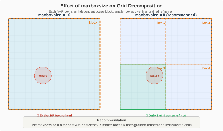
The simplest approach to building a single level uniform grid.
  grid
  {
    number of levels       = 1
    max box  size          = 8
    first level dimension  = [256^3]
    domain min             = [0., 0., 0.]
    domain max             = [ 1.,  1., 1.]
  }
Here we define a grid of 256 cells in each spatial dimension on a 3D domain, resulting in a uniform grid with \(256^3 = 16,777,216\) cells in total. The domain extends from \([0,0,0]\) to \([1,1,1]\), and with a box size of 8, each box contains \(8^3 = 512\) cells. Since only one refinement level (number of levels = 1) is specified, the entire grid maintains a uniform refinement level throughout the domain. It's important to note that first level dimension must evenly divide by max box size. If specifying a non-cubic domain (or non-square in 2-dimensions) grids the cells must remain cubes, so \(dx = dy = dz\). We also showcase a common shorthand used in input files, where [256^3] is equivalent to explicitly writing out [256,256,256].
While we have not yet discussed how to refine specific regions, it can sometimes be desirable to specify a minimum grid spacing explicitly. This can be achieved in two ways:
The first method (Option 1: Specify based on finest level) is by specifying finestdx. Setting finestdx explicitly limits the grid spacing to a minimum allowable value, ensuring refinement does not exceed this specified resolution:
The second approach (Option 2: Specify based on coarsest level) is to control refinement through the number of levels (number of levels). Each successive refinement level decreases the grid spacing by a factor of two relative to the previous level. The cell spacing (dx) at a given refinement level can be computed by
The following diagram illustrates how refinement levels relate to each other with a refinement ratio of 2:
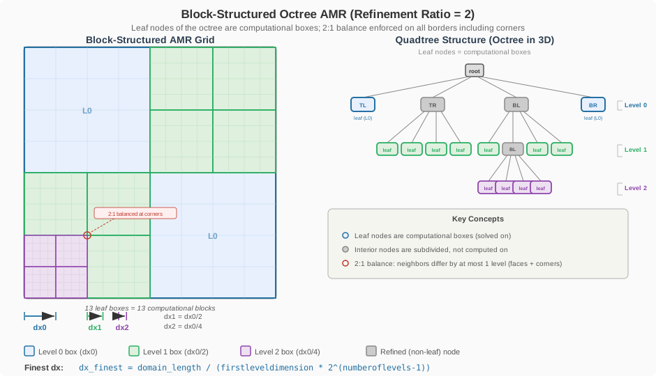
The following diagram illustrates the four tagging methods available for targeting refinement to specific regions of the domain:

Component Tagging
Specific refinement regions can be defined using component tagging based on the component numerical values from the input geometry. For example:
In this example, setting dx = 0.0 automatically applies the finest mesh resolution available, defined either by finestdx or the maximum number of refinement levels.
Tag Boxes
Refinement can also be targeted within explicitly defined rectangular regions (tagboxes):
This specifies a rectangular region from lo to hi coordinates, refined to a grid spacing (dx) of 0.4.
Tag Cylinders
Cylindrical refinement regions can be defined using the tagcylinders parameter. Each cylindrical region is specified with the following parameters:
tagcylinders_1 { lo = [0, 0, 0]; hi = [3, 0, 0]; radius = 2.24517; radius hi = 3.367785; dx = 0.0325 }
lo: Coordinates of the cylinder's bottom center point.hi: Coordinates of the cylinder's top center point.radius: Radius at the cylinder's bottom (lopoint).radiusinner: Inner radius at the cylinder's bottom, defining a hollow cylindrical region. Defaults to0.0if not specified.radiushi: Radius at the cylinder's top (hipoint). Defaults to the bottom radius (radius) if not specified.radiushiinner: Inner radius at the cylinder's top, defining the upper inner radius of a hollow cylindrical region. Defaults to the bottom inner radius (radiusinner) if not specified.
Tag Points
Pointwise tagging can also be utilized (remember, the entire box will be subject to the smallest tagged cell).
For all the above examples, each had an _1. This was because it was the first tagcylinder, box, etc. You can use any combination of these options or multiple of each. Each subsequent tag region of each type will just have to be incremented by +1 as shown in the tagpoints.
Instead of directly specifying dx, you may use dx_rel, a relative spacing factor multiplied by the reference dx (defined in the reference section).
Advanced Octree Grid Setup
The LAVA Cartesian solver uses block-structured AMR, where the domain is divided into boxes of \(8^d\) cells (shown as orange dashed boundaries in the diagrams below). There are two approaches for specifying grid resolution: Option 1 starts from the finest cell size and lets the solver determine the grid hierarchy, while Option 2 starts from the coarsest level dimensions and computes the finest resolution from the number of levels.
Here is user documentation for all grid section input options handled by LAVA Cartesian.
The grid section configures the AMR grid and domain setup. All options below are supported:
Option 1: Specify based on finest level
If you specify finestdx or finestdx_rel, the solver will automatically determine the number of refinement levels and grid dimensions to achieve the requested finest cell size.
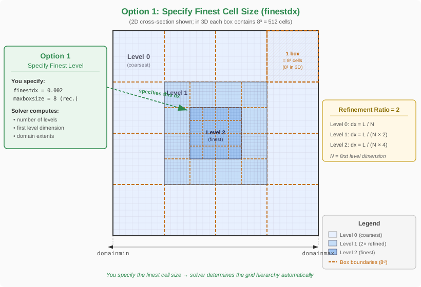
grid {
    finestdx = 0.002
    grid_scale = 1.0                                 # Optional: scales all grid lengths
    targetrelativefarfielddistance = [100, 100, 100] # Optional: domain size relative to reference length
    targetfarfielddistance = [100, 100, 100]         # Optional: absolute domain size
    domainorigin = [0.0, 0.0, 0.0]                   # Optional: domain origin
    aligndomainfacetoorigin = [none, lo, hi]         # Optional: align domain faces to origin per direction
    maxboxsize = 8                                   # Recommended: 8 cells per box side
                                                     #             (8³ = 512 cells/box in 3D)
}
finestdx: Target finest cell size (required for minimal input).finestdx_rel: Replaces finestdx if present. Target finest cell size factor relative to the referencedx(defined in the reference section).targetrelativefarfielddistance: Domain size relative to reference length (overridestargetfarfielddistanceif present).targetfarfielddistance: Absolute domain size.domainorigin: Domain origin.aligndomainfacetoorigin: Align domain faces to the origin; options per direction:none,lo, orhi.grid_scale: Scales all grid lengths (default: 1.0).maxboxsize: Maximum number of cells per box per direction. Recommended value: 8 (i.e., \(8^3 = 512\) cells/box in 3D). Must be at least 4 if using refinement.
Option 2: Specify based on coarsest level
Alternatively, you can specify the grid dimensions and number of levels directly:
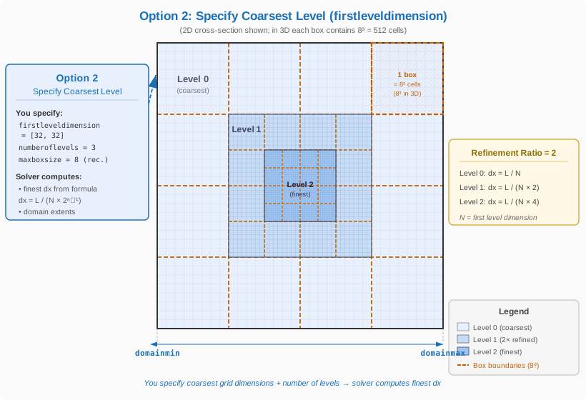
grid {
    firstleveldimension = [128, 128, 128]  # Number of cells in each direction on the coarsest grid
    numberoflevels = 3
    domainmin = [0.0, 0.0, 0.0]
    domainmax = [1.0, 1.0, 1.0]
    maxboxsize = 8                         # Recommended: 8 cells per box side (8³ = 512 cells/box in 3D)
}
firstleveldimension: Number of cells in each direction on the coarsest grid (must be a multiple ofmaxboxsize).numberoflevels: Number of AMR levels.domainmin,domainmax: Physical extents of the domain.maxboxsize: Maximum number of isotropic Cartesian cells per box, per direction. Recommended value: 8.
Additional Options
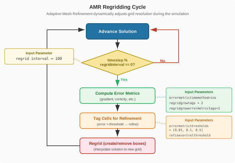
dumpinitgridsonly: If true, only writes initial grid and exits.regridinterval: Number of steps between regridding operations.regridintervalon,regridintervaloff: Control regridding intervals for on/off cycles.
regridgrowtags,regridgrowerrormetrictags: Control tag growth for regridding.
Notes
- All grid dimensions must be integer multiples of
maxboxsize. - For periodic boundary conditions, at least 2 boxes per direction are required.
- The refinement ratio between levels is fixed at 2.
- If the aspect ratio of cells is not unity and
nonunitokis not set, the code will stop with an error. We only support isotropic cells. maxboxsizemust be at least 4 if using refinement.
Adaptive Mesh Refinement Setup
The Cartesian solver supports solution-based AMR tagging using a variety of error metrics and field-based thresholds. These options allow you to refine the mesh dynamically in regions where the solution exhibits sharp gradients or other features of interest.
Solution-Based Adaptive Mesh Refinement
The solution based amr {} subsection enables solution-based AMR using a variety of error metrics. The available input options are provided below:
methodAMR thresholding method. Options include:user: Users must provide thresholds viaerrormetricthresholdfinestorerrormetricthresholds.auto: Refinement and coarsening thresholds are automatically determined using distribution thresholding.-
none: Solution-based AMR is turned off. -
errormetricthresholdfinestSet fixed error metric threshold per level based on the value for which the mesh should be refined to the finest available. The thresholds for coarsening and refinement for each level will then be automatically populated using the ratio to obtain the next coarsest refinement levelerrormetricthresholdratiowhich defaults to 0.5 to reduce mesh size as much as possible with minimal impact to solution accuracy -
errormetricthresholdminMin allowed threshold for solution based amr tagging. This is to avoid chasing non-physical error metrics. Default is 0.001. -
errormetricthresholdsSet fixed error metric thresholds per level (overrides the above if present). -
thresholddomainextentSpecifies whether to use the maximum or mean error as the maximum possible threshold value. Options:maxerror(use max error as the upper bound of threshold domain, default)meanerror(use mean error as the upper bound of the threshold domain)
-
maxcellsMaximum total number of cells. This limit is enforced when either user-specified thresholds or automated distribution thresholds are estimated to result in a total cell count exceeding the number specified. Example:maxcells = 150000000. -
maxcellstoleranceThe convergence criteria for the max cells constraint. For example, if 0.01 is specified, then we terminate the search when we have a set of thresholds that are 1% below the specified cell limit. Default:0.015. -
maxitercelllimitsearchThe maximum number of iterations to perform when searching for error thresholds that satisfy the imposedmaxcellsconstraint. Default:50. -
maxmemorypercenthostThe maximum percentage of host memory to utilize. This parameter is used at each adaptation cycle to generate an approximate limit on the number of cells we can afford to increase our grid size by. Default:80. -
maxmemorypercentgpuThe maximum percentage of GPU memory to utilize. This parameter is used at each adaptation cycle to generate an approximate limit on the number of cells we can afford to increase our grid size by. Default:80. -
enforcemaxmemorylimitAdjusts the user-specifiedmaxcellsparameter if memory usage will exceedmaxmemorypercenthostandmaxmemorypercentgpu. Warning this capability is currently under development and may result in undesired behavior. Default:false. -
errormetrictimemethodControls how error metrics are accumulated in time. Options:ins(instantaneous, default)avg(time average)max(maximum over time)
-
errormetricexponentialmovingaveragewindow,errormetricexponentialmovingaveragewindowctuWindow length for the exponential moving average (used iferrormetrictimemethod = avg). Thectuvariant is in convective time units; without the suffix the value is in physical time (seconds). -
errormetricresetonregridIf true, resets error metrics on each regrid. -
errormetricradialscalepoint,errormetricradialscalepowEnable and control radial scaling of error metrics. -
errormetricgeomdistancescalingreflengthReference length (\(d_0\)) for geometric distance scaling in error metrics, in meters. Scales down the error metric computed by \(1/2^{d/d_0}\) to avoid refining wakes and bow shocks all the way to the edge of the computational domain where they likely no longer affect quantities of interest. -
errormetricdogpuIf true, compute error metrics on GPU (requires at least one threshold to be set). -
errormetricstatsintervalInterval (in steps) to update error metric statistics
Notes:
- If the solution based amr section is NOT present, then no solution-based AMR is performed.
- If solution based amr is present, then the default for method is auto.
Specifying Error Metrics
The specification of error metrics is achieved through enumerated subsections errormetric_* {} within the solution based amr {} subsection. For example, two error metrics may be specified as follows:
grid
{
  solution based amr
  {
    errormetric_1 {type = laplacianp; weight = 0.5}
    errormetric_2 {type = laplaciant; weight = 0.5}
  }
}
Options include:
typeError metric name. Default:smallscaleenergy.weightWeight to apply to the specified error metric across all levels. Default: 1.0weightsperlevelArray of length equal to the number of AMR levels, specifying the weight to use on each level. If bothweightandweightsperlevelare provided, thenweightsperlevelwill be used. Default: [1.0,1.0,...,1.0]
Types of error metrics:
-
laplacianpRefine based on the Laplacian of pressure. -
laplacianu,laplacianv,laplacianwRefine based on the Laplacian of velocity components (u, v, w). -
laplaciant(single phase only) Refine based on the Laplacian of temperature. -
smallscaleenergyRefine based on small-scale energy content. -
vortrelRefine based on relative vorticity magnitude. -
tkeRefine based on turbulent kinetic energy (TKE). -
prmsRefine based on pressure RMS. -
maxmixing(multispecies only) Refine based on maximum mixing fraction.
Basic AMR Setup - User-specified Thresholds
    grid {
        finest dx = 0.008 # finest level based approach
        targetrelativefarfielddistance = [200,100^2]  # distance from origin to farfield BC in units of reference length
        aligndomainfacetoorigin = [none, none, none]
        max box size = 8
        regrid interval = 100 # number of time steps between regrids, larger is better for performance
        regridgrowtags = 2 # increases amount of refined boxes around geometry by 2 cells

        solution based amr
        {
          method = user
          errormetric_1 {type=smallscaleenergy; weight=1.0}
          errormetricgeomdistancescalingreflength = 22.5
          errormetricthresholds = [0.0000125, 0.000025, 0.00005, 0.000125, 0.00025, 0.0005, 0.00100, 0.0025, 0.005, 0.01, 0.04, 0.12, 0.24, 0.48, 0.96]
          regridgrowerrormetrictags = 1
        }
    }
Basic AMR Setup - Automatic Thresholds
    grid {
        finest dx = 0.008 # finest level based approach
        targetrelativefarfielddistance = [200,100^2]  # distance from origin to farfield BC in units of reference length
        aligndomainfacetoorigin = [none, none, none]
        max box size = 8
        regrid interval = 100 # number of time steps between regrids, larger is better for performance
        regridgrowtags = 2 # increases amount of refined boxes around geometry by 2 cells

        solution based amr
        {
          method = auto
          errormetric_1 {type=smallscaleenergy; weight=1.0}
          errormetricgeomdistancescalingreflength = 22.5
          regridgrowerrormetrictags = 1
        }
    }
Advanced Threshold-Based Refinement Inputs
All thresholds are specified as arrays of length equal to the number of AMR levels (except the base level). You may specify any combination of the following:
refineypluscomps = [ 1-9, 10]components to use for y-plus based refinementrefineyplusthreshold = [1000^9,200]yplus threshold levels for the components
Usage Notes
- You may specify any subset of the above thresholds; only those present will be used for refinement.
- Each threshold array must have length at least equal to the number of AMR levels.
- If no thresholds are specified but cell/target counts are set, the code will use default Laplacian-based refinement.
- For multiphase or multispecies cases, additional options are available as shown above.
Inputs Updating and Schedule Files
The inputs updating {} section lets you re-read the main input file during a run so you can tweak settings on the fly instead of stopping and restarting. On top of this manual workflow, you can optionally attach a schedule file to automate changes (e.g. ramping AMR levels, dx, CFL, or scheme order) within a single simulation as the flow evolves.
inputs updating block
The inputs updating section is defined at the top level of the input file (outside cartesian {}):
inputs updating {
  interval        = 1000           # how often to re-read the schedule
  do schedule     = true           # enable scheduling
  schedulefile    = schedule.dat   # relative or absolute path
  trigger         = ctu            # nt | time | ctu

  do cfl                 = false   # schedule CFL number
  do dt                  = false   # schedule explicit time step
  do levels              = true    # schedule number of AMR levels
  do max cells           = false   # schedule AMR cell-count cap
  do ref dx              = false   # schedule reference dx (dx-based regime)
  do order               = false   # schedule convective scheme order
  do upwind blending min = true    # schedule minimum upwind blending
}
interval: The time step interval of which the inputs file will be completely read again.do schedule: Switch for scheduling.schedulefile: Name/path of the schedule file.trigger:nt: schedule is keyed on time step number.time: schedule is keyed on physical time (seconds).ctu: schedule is keyed on convective time unitsdo cfl/do dt/do levels/do max cells/do ref dx/do order/do upwind blending min:- These booleans specify which quantities are controlled by the schedule file.
Schedule file format
The schedule file is a plain whitespace-separated table of numbers with no header or comments. Each row has the form:
The presence of each column are determined entirely by the inputs updating do ... bools:
The first column is always the trigger value. Subsequent columns appear only if the corresponding do ... flag is true, and always in this fixed order:
1. do cfl → CFL (cfl)
2. do dt → time step (dt)
3. do levels → number of grid refinement levels (levels)
4. do max cells → maximum total AMR cells (maxcells) for threshold based AMR
5. do ref dx → reference spacing (ref.dx)
6. do order → convective scheme flux order
7. do upwind blending min → convective terms { upwind blending min = ... }
For example, if you choose trigger = ctu, do levels = true, and do upwind blending min = true, each row has three columns:
To see a tutorial that utilizes scheduled inputs see the High Lift Prediction Workshop 5 (HLPW5) Common Research Model–High Lift (CRM-HL) case, which uses a schedule file to run a grid refinement study in a single run.
Initial Conditions
Initial condition specification is optional. If not provided, the code will simply initialize the flow to reference conditions specified in Reference Conditions.
If a different initialization is needed, it can be specified through a numbered list:
# Specify pressure, set the rest using reference conditions
IC_1 {pressure = 5e5}
# Specify temperature, set the rest using reference conditions
IC_2 {temperature = 500}
# If density is specified, another thermodynamic quantity (either pressure or temperature)
# also needs to be specified
IC_3 {density = 2; temperature = 300}
# Velocity vector can be specified
IC_4 {velocity = [100,10,0]}
# Or Mach number along with alpha and beta angles
IC_5 {Mach=0.5; alpha=6; beta=2}
# Specify mass fractions for multi-species
IC_6 {mass fractions = [1,0,0]}
All the above statements will apply the conditions listed in the entire domain. To initialize a sub-volume differently, you can specify a custom box region with position vectors of the two opposing corners:
The example above will first apply the reference conditions in the entire domain. Then it will overwrite the pressure in the unit box region specified. The IC's are applied sequentially, i.e. the entries further down in the IC's list will overwrite the previous ones if there is overlap.Near-Geometry Stagnation Initialization (Robust Startup)
For immersed-boundary simulations, all cells in boxes near the geometry can be initialized to stagnation (total) conditions using the near geom stagnation option. The purpose of this initialization is to soften the startup by zeroing out the velocity near the geometry and adjusting pressure and temperature to their total (stagnation) values, which can significantly improve robust startup behavior during the initial transient. It computes:
Optionally, corner_1 and corner_2 can be specified to restrict the stagnation initialization to a sub-region of the domain. Without them, the stagnation transform applies to all near-geometry cells in the entire domain:
When near geom stagnation = true is set on an IC block, no other thermodynamic or velocity parameters are allowed in that block — the base state comes entirely from the reference conditions.
Not supported for multiphase
IC Ordering Matters
IC blocks are evaluated in numbered order. A stagnation IC is only activated when both conditions are met: the cell is near the immersed geometry and it is within the stagnation IC's box bounds (the entire domain if no corners are specified). If either condition is not satisfied, the stagnation IC is skipped and the remaining IC blocks continue to be evaluated. Once a stagnation IC activates, it converts the current base state to total conditions and no further ICs are checked.
Stagnation IC listed first (recommended for most cases) — near-geometry cells within the stagnation box get stagnation conditions. All other cells skip the stagnation IC and fall through to subsequent ICs:
# Near-geometry cells get stagnation; all others skip this IC
IC_1 { near geom stagnation = true }
# Non-near-geometry cells (and those outside the stagnation box) can still receive custom conditions
IC_2 { pressure = 1e4; temperature = 300; velocity = [20,20,0]; corner_1 = [-2,-2,0]; corner_2 = [0,0,0] }
Stagnation IC listed last — custom ICs are evaluated first. Cells that match a custom box region receive those conditions and stop. Near-geometry cells that didn't match any earlier IC receive stagnation conditions based on the reference state:
# Custom conditions applied first in the box region
IC_1 { pressure = 1e4; temperature = 300; velocity = [20,20,0]; corner_1 = [-2,-2,0]; corner_2 = [0,0,0] }
# Near-geometry cells not matched above get stagnation of reference state
IC_2 { near geom stagnation = true }
Stagnation IC with corners — restricts the stagnation initialization to a specific region. Only near-geometry cells inside the specified box receive stagnation conditions; near-geometry cells outside fall through to subsequent ICs:
# Only near-geometry cells within this box get stagnation
IC_1 { near geom stagnation = true; corner_1 = [-0.5,-0.5,0]; corner_2 = [1.5,0.5,0] }
# Near-geometry cells outside the stagnation box, and all other cells, receive these conditions
IC_2 { pressure = 1e4; temperature = 300; velocity = [100,0,0] }
Info
The thermodynamic condition description for multi-phase is slightly different than for single and multi-species. Please refer to the Cartesian Multiphase Solver page for details.
Restarting
To resume runs, all you need to do is point to the restart file location as:
The restart files (also referred to as checkpoint files) are saved periodically in restart directory created by the code under the run directory. The interval at which the restart files are created can be specified by users. The details are provided in restart output options section.
If the specified restart file is not found, the solver will print a message and proceed with a fresh start instead of aborting. This allows the same input file to be used for both initial runs and restarts — if the restart file does not yet exist, the simulation simply starts from scratch. If restart is not desired at all, you can skip or comment out this section.
Additional restart controls are:
restart {
    file = ./restart/Cart_restartLatest.hdf5
    # Set physical time to 0 on restart
    reset time = true
    # Set the time step number to 0 on restart
    reset nt   = true
}
Boundary Conditions
Immersed Boundary Conditions
The LAVA Cartesian solver uses the Ghost Cell Method (GCM) for immersed boundary treatment, where ghost cells inside the body are assigned interpolated values from the fluid side to enforce boundary conditions. For details on the GCM approach, see Mittal et al.2 and for how we deal with thin geometry see Nakahashi et al.3.
Available types are: wall, inlet, nozzle,distributed, ref.
Available wall kinds are: no-slip,slip,wmpartialslip,porous,adiabatic,isothermal,wallstressmodel,musker,reichardt,blendedlog,wmnoslip,rough,roughrandom,wmslip,wmisothermal.
Available inlet kinds are: mdot,nozzle
Multiple kinds are possible for certain combinations, for example our recommended Immersed BC for WMLES:
The shorthand below is equivalent (when no velocity kind is specified,slip is assumed automatically; specifying wmpartialslip without wallstressmodel auto-adds wallstressmodel):
The available velocity treatments at an immersed wall are:
no-slip: classical Dirichlet (u = u_body) at the wall. Used for fully wall-resolved viscous simulations.slip: inviscid wall (u·n = u_body·n, tangential Neumanndu_t/dn = 0).wmpartialslip: wall-model-based partial slip. The immersed-boundary ghost-cell tangential velocity is determined by a linear reconstruction through the matching point (at off-wall distanced1) and the wall-model profile value at y⁺ =partialslipheight(default 100, deep in the log layer). This is an attempt at making the tangential velocity wall-normal gradient for the convective terms more consistent with the viscous stress correction that uses the wall function predicted wall shear stress. No wall-normal velocity is still imposed as inslip(u·n = u_body·n). When the transition sensor detects laminar flow ortau_w ≈ 0, the BC collapses tono-slip. Requireswallstressmodeland a wall-model law (blendedlogis the default).
Where, the wall stress model options include:
    # Pick wall function, kind options: musker (default), reichardts, blendedlog, rough
    kind = blendedlog
    # If using rough wall model, specify the roughness in meters
    # 0.25e-6m : highly polished
    # 0.50e-6m : polished
    # 3.33e-6m : painted
    roughness = 0.5e-6
    # Anchor y+ for wmpartialslip reconstruction (y+ units, default = 100)
    partialslipheight = 100
mdot Immersed Boundary Condition:
This boundary condition allows the user to prescribe the inflow with thermodynamic conditions, and mass flow rate. A sample setup is shown below:
  type            = inlet
  kind            = [mdot]
  mdot            = 193.1277 # Mass flow rate in kg/s
  area            = 0.162647 # Injection area in m2 (3D) or m (2D)
  #pressure        = 1e5 # Optional pressure parameter
  temperature     = 300
  massfractions   = [0.992442,1e-8,1e-8,0.007558] # If running with MS
  components      = [2] # List of components to apply this BC
pressure parameter can be prescribed to enforce a pressure along the inlet. This can be useful to model over/underexpanded inlet flows. However, for such configuration, it is recommended to use the nozzle boundary condition instead. When pressure is not prescribed, the solver will extrapolate pressure from the interior.
Info
To easily switch between 3D and 2D modes, mdot and area can be kept the same, since only their ratio is considered in the code.
Info
The thermodynamic condition description for multi-phase is slightly different than for single and multi-species. Please refer to the Cartesian Multiphase Solver page for details.
nozzle Immersed Boundary Condition:
The nozzle boundary condition is mainly used for launch simulations where the boundary condition is applied to the nozzle exit. It also comes with a few physics options to improve stability and control the output. A basic boundary condition can be specified via the following:
where the nozzle boundary condition takes an input file filename which has several supported file types datafiletype described below. Like the above boundary conditions, they are applied to a component on the triangulation specified by components. In a multispecies simulation, you must also specify ispecies which corresponds to the 0 based index of the mixture in the fluid section for which species the nozzle will eject.
A complete list of all the options is provided below, along with default options where applicable:
Main Options:
| Variable | Description |
|---|---|
| filename | (Required) The filename of the describing boundary condition file |
| datafiletype | (Required) The type of datafile. 0 is a steady (constant) ascii file. 1 is radially varying constant ascii file, 2 is unsteady but constant in space ascii file, 3 is unsteady radially varying binary, 4 is unsteady radially varying ascii file |
| ispecies | (Required for multispecies/multiphase) Specifies the component of mixture for the nozzle to eject. |
| nozzlecenter | (Optional) Specifies the coordinates of the nozzle center |
| nozzlenormal | (Optional) Specifies the normal for the boundary condition to be applied on |
| asciilinetimestart | (Required) Only used for datafiletype=4. Specifies the line number to start reading the file. |
| asciilinetimestop | (Required) Only used for datafiletype=4. Specifies the line number to stop reading the file. |
| asciilinetimeskip | (Optional) Only used for datafiletype=4. Specifies the stride at which to read lines from the file. Default is 1. |
| asciilinereadspecies | (Optional) Only used for datafiletype=4. Bool for whether this file contains species information as well. Default is false. |
| numberofradialpoints | (Required) Only used for datafiletype=4. Specifies the number of radial points in the file. |
Note
The mixture state prescribed when asciilinereadspecies=true takes precedent over ispecies. In this case, ispecies is disregarded by the reader.
Ramp Options:
| Variable | Description |
|---|---|
| rampsteps | (Optional) Will linearly warmup the nozzle based on rampsteps number of timesteps by taking a linear combination of the reference Q and the user specified conditions in filename. Default is 0 (no step ramping). |
| rampnton | (Optional) The timestep number to turn the ramping on. Nozzle will be off prior to this timestep. (Only used with rampsteps). Default is -1. |
| ramptimestart | (Optional) If rampsteps is not turned on, the other ramping option is using simulation time. This is the same linear warmup between ramptimestart and ramptimestop. Before ramptimestart the nozzle is off if it is specified. Default is no time ramping. |
| ramptimestop | (Optional) The simulation end time to ramping. |
| timeshift | (Optional) Timeshift can be used to shift the nozzles in time relative to the simulation time. This is compatible with ramping. Default is 0. |
Note
One should only use (rampsteps and rampnton) or (ramptimestart and ramptimestop). They will not work in a combined fashion.*
Physics Options:
| Variable | Description |
|---|---|
| multiphaseequilibrium | (Optional) Only used in cartesian + multiphase. This computes multiphase equilibrium on the boundary condition. Default is false. |
| dostagnation | (Optional) Apply stagnation inlet boundary conditions. Not supported for multiphase. Default is false. |
| doautomaticsonicinlet | (Optional) Only used when dostagnation = false. If the boundary condition goes below subsonic speed, we get pressure from the interior. This keeps the velocity at the inlet >= mach 1. Not supported for multiphase. Default is false. |
| dothroatsonicinlet | (Optional) Only used when dostagnation = true. Forces the pressure to be sonic + 1%. Not supported for multiphase. Default is false. |
ASCII Data Format
datafiletype = 0 or 1: steady, radially constant or varying, ascii file: radius(m) Pressure(Pa) Temperature(K) u_normal(m/s) u_radial(m/s)
datafiletype = 2: unsteady, radially constant, ascii file: time(s) Pressure(Pa) Temperature(K) u_normal(m/s) u_radial(m/s)
Info
Lines starting with # are omitted by the parser for datafiletype = 0, 1, 2.
datafiletype = 4: unsteady, radially varying, ascii file: line_number time(s) radius_x(m) radius_y(m) [radius_z(m)] Pressure(Pa) u_normal(m/s) u_radial(m/s) [u_azimuthal(m/s)] Temperature (m) [Species Mass Fractions]
Note
The format of datafiletype = 4 depends on the dimension of the configuration. The extra fields radius_z(m) and u_azimuthal(m/s) are required when running with 3D and must be omitted when running with 2D. Currently, the field u_azimuthal(m/s) is disregarded in the nozzle bc, however, it must still be present in the nozzle data file. Also, the fiels Species Mass Fractions are only present when asciilinereadspecies = true. Also, note that no comments are allowed in this file type format.
An example of a type-4 nozzle data base is shown below for the configuration asciilinetimestart = 0; asciilinetimestop = 30; asciilinetimeskip = 10; asciilinereadspecies = true:
  0   -10000  0.000 0 0  10000  1000   0  0    1500  0. 0. 1. 0.
  0   -10000  0.500 0 0  40000  1000   0  0    1500  0. 0. 1. 0.
  0   -10000  1.000 0 0  80000  1000   0  0    1500  0. 0. 1. 0.
  0   -10000  1.965 0 0 110000  1000   0  0    1500  0. 0. 1. 0.
  10   1.000  0.000 0 0  10000  1000   0  0    1500  0. 0. 1. 0.
  10   1.000  0.500 0 0  40000  1000   0  0    1500  0. 0. 1. 0.
  10   1.000  1.000 0 0  80000  1000   0  0    1500  0. 0. 1. 0.
  10   1.000  1.965 0 0 110000  1000   0  0    1500  0. 0. 1. 0.
  20   10000  0.000 0 0  10000  1000   0  0    1500  0. 0. 1. 0.
  20   10000  0.500 0 0  40000  1000   0  0    1500  0. 0. 1. 0.
  20   10000  1.000 0 0  80000  1000   0  0    1500  0. 0. 1. 0.
  20   10000  1.965 0 0 110000  1000   0  0    1500  0. 0. 1. 0.
  30   20000  0.000 0 0  10000  1000   0  0    1500  0. 0. 1. 0.
  30   20000  0.500 0 0  40000  1000   0  0    1500  0. 0. 1. 0.
  30   20000  1.000 0 0  80000  1000   0  0    1500  0. 0. 1. 0.
  30   20000  1.965 0 0 110000  1000   0  0    1500  0. 0. 1. 0.
Domain Boundary Conditions
Absent user inputs, the farfield domain boundary conditions are set automatically based on reference conditions (e.g. Reynolds, Mach, temperature, alpha, beta).
We recommend using the automatically generated farfield boundary conditions for most external flow cases, when used with typical CFD best practices (domain should extend 50-100 body lengths in each direction).
However, for internal flows or half-span models, it may be necessary to specify farfield boundary conditions manually.
The 6 domain face boundary conditions are specified as follows, where type and kind are given. Each entry in the arrays corresponds to the x, y, and z directions respectively (index 0, 1, 2). The lo arrays define the boundary condition on the minimum face of each direction, and hi on the maximum face.
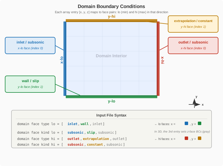
domain face type lo = [inlet    ,wall         , inlet]
domain face kind lo = [subsonic ,slip         , subsonic]
domain face type hi = [outlet   ,extrapolation, outlet]
domain face kind hi = [subsonic ,constant     , subsonic]
inlet, wall, outlet, extrapolation, ref, periodic.
Available inlet kinds are: subsonic,mdot
Available wall kinds are: no-slip,slip
Available outlet kinds are: subsonic
Available extrap kinds are: constant,linear
For half-span models, the equivalent mirror boundary condition type is wall with kind slip. Periodic boundary conditions are supported but not recommended for thin strips of airfoils or wings because it severely limits the ability to coarsen away from the airfoil: due to its forest of octree design, we currently require at least 3 boxes across the smallest domain direction on the coarsest level. If thin periodic airfoils/wings is your primary use case, we suggest using LAVACurv or LAVAUnst as they are better suited to this type of task.
Trip Lines
Trip lines exert a penalty method source term that attempts to trigger boundary layer transition to turbulence. The source terms are applied only at select cells within certain distance of the lines. Lines are also broken into dash/dot or on/off pattern that apply the trip terms in an intermittent fashion along the line, similar to how trip dots are commonly implemented in reality.
# This determines the strength of the trip lines
# The lower the value, the stronger the trip source penalties are
# In the lower limit, a value of 1 would bring the flow to full stop
# where trip is active
trip time relaxation = 40. # a factor of dt
trip_line_1 {
    # dxscale should indicate the local grid resolution (where this trip line is)
    # with respect to the dx value set at the reference section
    dxscale = 1
    # Begin/end coordinates of the line segment
    begin = [0,1,1]
    end   = [1,2,3]
    # The segment variables below are relative to the local grid spacing
    # In this example, the trips will be on for approximately 2 cells
    # and off for approximately 3 cells along the line
    # The on segments will mark cells whose centers are within 0.9 * dx
    # from the line
    # These variables can be skipped in favor of defaults
    segment length = 2 # default
    segment skip   = 3 # default
    segment radius = 0.9 # default
    # The straight trip line specified here will be projected to the
    # surface using projection method. By default, the line will be projected
    # to the closets surface
    # Options are : none, closest, vector
    projection method = closest # default
    # max distance is an optimization parameters, entering the something
    # slightly larger than the expected farthest distance (from trip line to the geometry)
    # will improve start-up performance
    projection max distance = 3
}
trip_line_2 {
    dxscale = 4
    begin   = [1,0,0]
    end     = [2,0,0]
    # Another projection method is vector, for which the line
    # is projected along a specified vector direction until a surface is
    # encountered
    projection method = vector
    projection vector = [0,1,0] # y-axis
}
# Circular trip curve
trip_line_3 {
    dxscale = 2
    # Instead of a straight line, the trip location can also be drawn as a circle
    # with the specified center coordinates and radius
    center  = [1,0,0]
    radius  = 2
    # The circle can also be projected to the surface
    projection method = closest
    projection max distance = 1
}
Tip
In typical practice, it is recommended to use defaults for segmenting parameters. In addition, the inputs may be made more compact by inlining each trip, for example:
Tip
The solver will output the final projected trip lines (in tecplot and vtk line formats) into the trips directory under the run directory. It is highly recommended to verify the trip setup by plotting the lines overlaid on the surface geometry.
Output
Flow Stats
Controls interval of sampling flow statistics such as integrated kinetic energy, maximum Mach number and integrated domain volume (see Monitor section for descriptions).
Loads
In this section, you can define several loads integration groups which can integrate forces and moments over specified components of the geometry.
output {
    loads {
        # Interval at which the loads are computed, this is common for all integration groups
        interval      = 10
        # Following 3 inputs apply to all the groups by default
        # But you can optionally specify them different for any individual group
        # Center around which moments are computed
        moment center = [33.,0.0,4.5]
        # Provide non-dimensional force and moments
        normalize     = true
        # Use gauge pressure (p-p_ref) in pressure forces
        gauge         = true
        # If true, this flag will output each surface component integrations separately
        # (in addition to the groups listed below)
        do individual comps = true
        group_1 {
            # Group name
            name          = airplane
            # Which BC zones to include
            include       = [1-32]
        }
        group_2 {
            name = wing
            include = [7,8,10-13]
            normalize     = false
            # Use gauge pressure (p-p_ref) in pressure forces
            gauge         = false
        }
        group_3 {
            name = tail
            include = [14,16]
            moment center = [48.,0.0,4.5]
        }
        ...
    }
}
normalize = true is specified, the code will additionally output normalized force/moment coefficients. Reference section values are used for normalization.
The result of the load integrations are output to screen (if requested) and to the monitor file (.iter). Detailed description of the monitor and the loads output variables are provided in the monitor section.
If you only have single loads integration group, you can skip the group_1 subsections:
output {
    loads {
        interval      = 10
        moment center = [33.,0.0,4.5]
        normalize     = true
        gauge         = true
        do individual comps = true
        name          = airplane
        include       = [1-32]
    }
}
Monitor
Monitor output tracks typically high frequency information such as time step, CFL, residuals, integrated aerodynamics loads and performance metrics among others.
If monitor section is not included in the input file, you will get a default set of variables output to screen every time steps (or every pseudo step for implicit runs). The variable list given here only affects the screen output while every other available variable is always output to the .iter file.
The .iter file can be plotted using the tool plotHist.py
output {
    monitor {
        # Output interval applies both to screen and file (.iter) file outputs.
        interval = 10
        # Variable list only affects the screen output
        variables = [nt,time,ctu,dt,maxcfl,maxmach,cl_airplane,wallt,mups,elapsed]
        # When restarting, the code looks for a copy of the .iter file in the restart directory
        # corresponding to the time step you are restarting from. If the .iter file is missing,
        # by default the code will quit with an error message. The flag below, if activated, will
        # instead start a new .iter file from scratch
        reset if missing = false # default
        # The monitor keeps track of some averaged performance metrics. This entry will set the interval
        # for averaging. By default, it is set to 10xinterval (specified above)
        avg interval = 100
    }
}
List of available monitor variables:
| Variable | Description | Units |
|---|---|---|
| nt | Time step | |
| ns | Pseudo time step | |
| time | Physical simulation time | [s] |
| ctu | Convective time unit | [non-dimensional time] |
| dt | Time step size | [s] |
| maxcfl | Maximum CFL number in the domain | |
| maxmach | Maximum Mach number in the domain | |
| integratedmass | Integrated mass of fluid in the domain | [kg] |
| integratedvolume | Integrated volume of the domain | [m^3] |
| integratedke | Integrated kinetic energy in the domain | [J] |
| nondim_integratedke | Non-dimensional integrated kinetic energy | |
| integratedxmomentum | Integrated x-momentum | [kg*m/s] |
| integratedymomentum | Integrated y-momentum | [kg*m/s] |
| integratedzmomentum | Integrated z-momentum | [kg*m/s] |
| integratedetotal | Integrated total energy in the domain | [ (kg/m^3)(m^2/s^2) ] |
| nondim_integratedetotal | Non-dimensional integrated total energy | |
| minpressure | min pressure in the domain | [Pa] |
| maxpressure | max pressure in the domain | [Pa] |
| minuvelo | min u-velocity in the domain | [m/s] |
| maxuvelo | max u-velocity in the domain | [m/s] |
| minvvelo | min v-velocity in the domain | [m/s] |
| maxvvelo | max v-velocity in the domain | [m/s] |
| minwvelo | min w-velocity in the domain | [m/s] |
| maxwvelo | max w-velocity in the domain | [m/s] |
| mintemperature | min temperature in the domain | [K] |
| maxtemperature | max temperature in the domain | [K] |
| mups | Average MUPS, averaged through the log interval | |
| mups_min | Minimum MUPS through the monitor log interval | |
| mups_max | Maximum MUPS through the monitor log interval | |
| mups_long | Average MUPS, averaged through the avg interval | |
| mups_long_min | Minimum MUPS through the monitor avg interval | |
| mups_long_max | Maximum MUPS through the monitor avg interval | |
| wallt | Wall time per time step, averaged through the log interval | [s] |
| wallt_min | Minimum wall time through the monitor log interval | [s] |
| wallt_max | Maximum wall time through the monitor log interval | [s] |
| wallt_long | Wall time (s), averaged through the avg interval | [s] |
| wallt_long_min | Minimum wall time through the monitor avg interval | [s] |
| wallt_long_max | Maximum wall time through the monitor avg interval | [s] |
| elapsed | Total elapsed wall time from beginning, including the restart history | [hr] |
| memory | CPU host memory usage on root MPI rank | [GB] |
| memory_gpu | GPU device memory usage on root MPI rank | [GB] |
Note
MUPS: Millions of Updates per Second, i.e. millions of cells advanced through a full time step per second
Integratrated loads, as described in the Loads section, are also output via the monitor. Each loads integration group, corresponding to the its specied name will produce the following monitor output variables:
| Variable | Description |
|---|---|
| cx_name | Total x-force coefficient |
| cy_name | Total y-force coefficient |
| cz_name | Total z-force coefficient |
| cx_inv_name | Inviscid x-force coefficient |
| cy_inv_name | Inviscid y-force coefficient |
| cz_inv_name | Inviscid z-force coefficient |
| cx_visc_name | Viscous x-force coefficient |
| cy_visc_name | Viscous y-force coefficient |
| cz_visc_name | Viscous z-force coefficient |
| cmx_name | Total x-moment coefficient |
| cmy_name | Total y-moment coefficient |
| cmz_name | Total z-moment coefficient |
| cmx_inv_name | Inviscid x-moment coefficient |
| cmy_inv_name | Inviscid y-moment coefficient |
| cmz_inv_name | Inviscid z-moment coefficient |
| cmx_visc_name | Viscous x-moment coefficient |
| cmy_visc_name | Viscous y-moment coefficient |
| cmz_visc_name | Viscous z-moment coefficient |
| cl_name | Total lift coefficient |
| cd_name | Total drag coefficient |
| cs_name | Total side force coefficient |
| cl_inv_name | Inviscid lift coefficient |
| cd_inv_name | Inviscid drag coefficient |
| cs_inv_name | Inviscid side force coefficient |
| cl_visc_name | Viscous lift coefficient |
| cd_visc_name | Viscous drag coefficient |
| cs_visc_name | Viscous side force coefficient |
Restart
Restart files, also referred to as checkpoint files, allow you to restart the simulation seamlessly from a given point. You can set the interval of restart file writes as:
output {
    restart {
        # Specify restart file output interval (time step for unsteady, pseudo-step for steady)
        interval = 1000
    }
}
Volume
The Cartesian solver writes volume output using parallel HDF5 output. The volume output is controlled with the following, where interval can be 0 for no output:
In addition to the full volume output, you can also output a subset of the domain using a box region. Each subset can have its own output interval that differs from the main volume interval.
volume {
     interval = 1000
     variables = [q,mach,density,mask,processor]

     subset_1 {
         type = box
         lo = [0.1, 0, 1.0]    # Minimum coordinates [x_min, y_min, z_min]
         hi = [1.0, 0.5, 0.1]  # Maximum coordinates [x_max, y_max, z_max]
         interval = 500        # Output interval specific to this subset
     }
     subset_2 {
         type = box
         lo = [-1.0, -0.01, -0.01]
         hi = [ 1.0,  0.01,  0.01]
         interval = 100
     }
   }
The variables input is shared across all subsets. Each subset can have its own output interval. Output files follow the naming convention sub01.Cart.XXXXXXXXX.hdf5, sub02.Cart.XXXXXXXXX.hdf5, etc. Thin box subsets can be used to approximate plane extractions.
The 3D block-structured box layout is also written to boxes_* files at the same frequency as interval. These files contain the outlines of all boxes in the domain and are primarily useful for visualizing the volume mesh structure.
Tip
For large simulations, using subsets can significantly reduce storage requirements and post-processing time.
Iso-Surfaces
In-situ extraction of iso-surfaces for post-processing and visualization is supported. Iso-surfaces are defined by specifying a contour value for a chosen field, and the solver will output the corresponding isosurface as a triangulation at a user-defined interval.
isosurfaces_1 {
    isovalue     = 0.5
    contour      = vortmag
    colorfield   = umag
    interval     = 100
    format       = vtk
    clipbox_1 {
        lo     = [0.0, 0.0, 0.0]
        hi     = [1.0, 1.0, 1.0]
        invert = false
    }
}
isosurfaces_2 {
    contour      = cutplane
    normal       = [0, 1, 0]         # Normal vector of the plane (e.g., y-normal)
    point        = [0.0, 0.5, 0.0]   # A point on the plane
    colorfield   = densitygradmag
    interval     = 100
}
isosurfaces_3 {
    contour     = cutplane
    point       = [9.75, 0, 0]
    normal      = [1, 0, 0]
    format      = vtk
    interval    = 100
    colorfield  = fullq
    derivedvars = [mach, density]
}
isosurfaces_4 {
    isovalue        = 300
    contour         = q
    qcompcontouring = 4 # temperature component of the q vector for 3D simulations
    colorfield      = q
    qcompcoloring   = 0 # pressure component of the q vector
    interval        = 100
    format          = vtk
}
Parameters
- isovalue: The value of the chosen field at which to extract the iso-surface (e.g.,
isovalue = 0.5). - contour: The field to contour. Options include:
vortmag(vorticity magnitude, default)qcriterionmachdensitygradmagq(a specific component of the q vector. The optionqcompcontouringis then required to specify the component index)cutplane(for planar cuts; requiresnormalandpoint)
- colorfield: Field used to color the iso-surface. Options include:
umag(color with velocity magnitude, default)vortmagqcriterionerrormetricdensitygradmagq(color with a specific component of the q vector. The optionqcompcoloringis then required to specify the component index. If the optionqcompcoloringis missing, thenfullqis used instead)fullq(color with all components of the q vector)
- interval: Output interval in time steps (e.g.,
interval = 100). - format: Output file format. Buffered Options:
vtk(default),vtp,cgns,fwh. Non-buffered options:xdmf,vtk,vtp.vtpwrites VTK XML PolyData (.vtp) files with raw binary appended data.
- cliplo, cliphi: (Optional, deprecated) Lower and upper bounds for spatial clipping of the iso-surface, specified as coordinate arrays. Defaults to the full domain. Equivalent to a single
clipbox_1 { lo=...; hi=...; invert=false }; emits a deprecation warning at run time. Cannot be combined with indexedclipbox_Nsub-sections. Preferclipbox_1in new inputs. - clipbox_N: (Optional) Indexed axis-aligned box clip(s). Up to 4 boxes are supported per iso-surface (
clipbox_1,clipbox_2, ...). Each box haslo,hi, and an optionalinvertflag (defaultfalse). Wheninvert=falsethe box keeps points inside it; wheninvert=trueit keeps points outside it. All configured boxes are AND'd together, and AND'd with allclipfrustum_Nregions. Example — keep points inside a large box but excluded from a small interior box: - clipfrustum_N: (Optional) Indexed frustum (or hollow frustum) clip(s). Up to 4 frustums are supported per iso-surface (
clipfrustum_1,clipfrustum_2, ...). The frustum axis runs fromlotohi;radiusis the cross-section radius atlo, and the optionalradiushiis the radius athi(defaults toradius, i.e., a cylinder). The optionalradiusinnerandradiushiinnercarve out a coaxial hollow region (defaults:0). An optionalinvertflag (defaultfalse) flips the keep/discard sense for that frustum: withinvert=truepoints inside the frustum are discarded. All frustums are AND'd together and AND'd with any box clips. Example — a hollow cylinder along the y-axis betweeny=0.1andy=0.4with outer radius0.18and inner radius0.08:isosurfaces_4 { isovalue = 10 contour = vortmag colorfield = umag interval = 100 clipfrustum_1 { lo = [0.75, 0.10, 0.50] hi = [0.75, 0.40, 0.50] radius = 0.18 radiusinner = 0.08 # radiushi = 0.18 # optional, defaults to radius (cylinder) # radiushiinner = 0.08 # optional, defaults to radiusinner # invert = false # optional, default false } } - normal, point: (Optional) For planar cuts, specify the normal vector and a point on the plane.
- qcompcontouring: Required for
contour = q, selects the q component to contour. - qcompcoloring: Required for
colorfield = q, selects the q component for coloring. - derivedvars : (Optional) For
colorfield = fullqorcolorfield=qwithout anyqcompcoloringspecification, the output state vector can be appended with derived variables. Available options are any combinations of:machdensity
Multiple Iso-Surfaces
You can define multiple iso-surfaces by incrementing the section name, e.g., isosurfaces_1, isosurfaces_2, etc.
Notes
- If
contour = cutplane, you must provide bothnormalandpoint. - If
format = xdmf, parallel output is enabled by default (only recommended for very large iso files). - If
colorfield = qandqcompcoloringis not specified, the full Q vector is used for coloring. - There is a parallel/serial option exposed to the user, but we recommend to not set that and allow the code to determine the best setting.
- Buffered output for isosurfaces is controlled by the
outputbufferintervalisos = 5000variable in the output section. No need to set that variable as the code will automatically determine a best buffering interval. - For
qcompcontouringandqcompcoloring, the component of the state vector follows this 0-index order: [p u v (w) T (Y1 Y2 Y3 ...)]. Here, note that the fieldwonly exists when running the 3D executable.
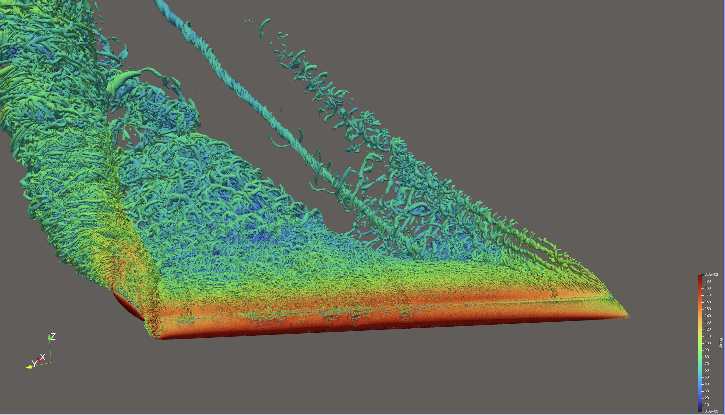
Example Q-Criterion output by the LAVA Cartesian AMR flow solver, colored by velocity magnitude for HLPW6 at alpha=35 degrees.
Surface
Surface Probes can be used to sample the flow on a plane slice.
output {
    surface probe_1 {
        cutpoint     = [0, 0.1, 0] # Origin of the cut plane
        cutdirection = y  # plane normal direction
        interval     = 10 # Interval of sampling
        datalocation = face # sample location (face or node)
    }
}
Cut planes are only supported for x, y and z normal planes.
The results will be written out to surf_probe directory. Each surface probe section will get its own file and will contain all the variables.
The output format can be selected with the format option. Available options include vtk (legacy VTK, default for Cartesian) and vtp (VTK XML PolyData). Example:
The Cartesian solver has the ability to buffer our surface output in such a way that all MPI ranks can do simultaneous parallel writes. This is controlled by the optional outputbufferintervalsurf = 20000 variable, where 20000 is an example time-step interval. If the variable is left out, the code will automatically compute the outputbufferintervalsurf if it is not provided.
Wall-model surface variables
In addition to the standard surface variables (q, mach, pcoef, etc.), the following per-vertex wall-model quantities can be requested in the surface variables list and are written when at least one immersed BC uses a wall-stress model:
tauwX,tauwY,tauwZ: components of the modeled wall shear stress vector.yplus:y+evaluated at the wall-model sample point.partialslip: dimensionless slip indicator in[0, 1]: ratio of the wall-model tangential velocity at y⁺ =partialslipheightto the tangential velocity at the wall-model sample point.1= fully slip (profile is nearly flat between y⁺ =partialslipheightand the sample point);0= no-slip (laminar flow detected by the transition sensor, ortau_w ≈ 0). Useful for visualizing where thewmpartialslipBC is operating in its slip-like vs. no-slip-like regime.qdot: surface heat flux. Automatically skipped if no isothermal/wmisothermalwall is present in the BC configuration (the value would be zero).turbulence: turbulence-transition sensor. Automatically skipped if no wall hastransitionthreshold > 0configured (the sensor is inactive).
All of the above are also enabled together via the shorthand token wallmodel in the variables list.
Surface Probe
User specified surface extractions are possible using either an arbitrary triangulation, or user specified cut-planes.
surface probe_1 {
     file        = triangulation.i.tri
     scale       = [0.75^3]
     interval    = 10
   }
surface probe_2 {
     cutpoint = [1,0,0]
     cutdirection = y
     interval     = 10
   }
surface probe_3 {
     cutpoint   = [-0.1,0,0]
     cutpointhi = [ 0.1,0,0]
     numplanes = 11
     cutdirection = x
     interval     = 10
   }
}
For cut-plane probes, boxes_* files are also written alongside the cut-plane output. These correspond to the block-structured boxes intersected by each cut-plane and are primarily useful for cleanly visualizing the box layout as intersected by the cut-plane without the visual overhead of full cell-level data. Each box also carries per-box scalar values as a secondary, lower-resolution representation of the flow solution.
Line Probe
lineprobe_1 {
    start = [-1.000, 0.0,0];
    end = [1.000,0.0,0];
    number of points = 512;
    interval = 20;
    }
Point Probe
Point probes will sample the flow state at a number of given points.
A group of points can be specified at once using an ascii file that lists the x y z coordinates of each point in order (space delimited):
output {
    point probe_1 {
        file = ascii_file_with_xyz_coords.dat
        interval = 1 # Interval of sampling
        scale = 1 # Option to scale the coordinates
    }
}
Results will be written to an ascii file in the point_output directory, where each probe section and each variable will get its own file.
References
-
Deng, X., "New High-Order Hybrid Cell-Edge and Cell-Node Weighted Compact Nonlinear Schemes," 20th AIAA computational fluid dynamics conference, 2011. https://doi.org/10.2514/6.2011-3857 ↩
-
R. Mittal, H. Dong, M. Bozkurttas, F. M. Najjar, A. Vargas, and A. von Loebbecke, "A versatile sharp interface immersed boundary method for incompressible flows with complex boundaries," Journal of Computational Physics, vol. 227, pp. 4825–4852, 2008. ↩
-
Nakahashi, Kazuhiro. "Immersed boundary method for compressible Euler equations in the building-cube method." 20th aiaa computational fluid dynamics conference. 2011. ↩