Multielement Airfoil RANS
The 2D multielement airfoil is a Reynolds-Averaged Navier-Stokes (RANS) verification case from the NASA Langley Research Center's Turbulence Modeling Resource. This case simulates flow over a 2D, high-lift configuration airfoil with slat, main and flap elements at \(\textrm{Mach}=0.2\), \(\textrm{Re}=5\times10^6\), and \(\alpha=16^{\circ}\).
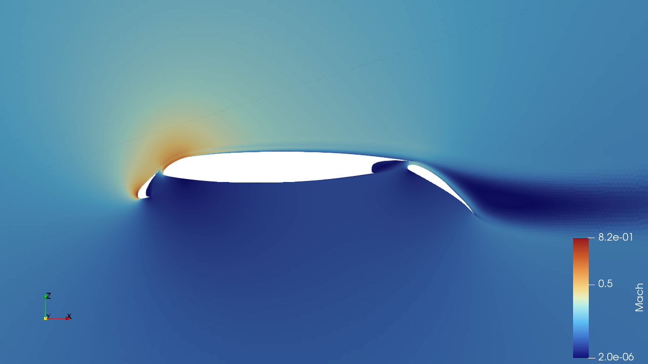
Mach number contours around the three-element high-lift configuration.
Prerequisites
Before starting this tutorial, ensure you have:
- LAVA solver installed and accessible — see LAVA Installation Guide
- LAVA Voronoi mesher installed — see Voronoi Installation Guide
- Basic familiarity with LAVA input file structure — see Unstructured Solver Inputs
Tutorial Files
Download the input files for this tutorial:
| File | Description |
|---|---|
| crmhl-2dcut-triangulation.cgns | Surface geometry triangulation |
| voro_mea2d.yml | Voronoi meshing input file |
| unst_mea2d.inputs | Solver input file |
Directory Setup
Create a working directory for this tutorial with separate folders for meshing and simulation:
Place the downloaded files in the appropriate folders:
voro_mea2d.yml→meshing/crmhl-2dcut-triangulation.cgns→meshing/unst_mea2d.inputs→run/
Meshing
The Voronoi meshing input for the multielement airfoil specifies a 1000m × 1000m domain. The three-element airfoil assembly (slat, main element, and flap) is positioned at the domain center. Anisotropic Voronoi cells are generated along the airfoil surfaces with a spacing growth rate of 1.25. Outside the anisotropic region, spacing transitions from fine to coarse through 8 cell-thick layers until the farfield is reached.
Note
LAVA unstructured solver does not support true 2D meshes. For 2D simulations, we create 3D meshes with a single cell in the depth direction.
Navigate to the meshing/ directory and generate the mesh:
Executable Names
The Voronoi executable name varies by architecture. See the Voronoi Installation Guide for details.
PBS Setup on NAS
If running on NAS systems, ensure that you have read the Running On NAS Guide for example PBS setup scripts.
This generates voro_mea2d.cgns in the current directory. Link this file to the run directory:
Note
The provided Voronoi input file will generate a coarser mesh than required for mesh insensitive results. You can reduce the reference_length parameter in the voro_mea2d.yml for finer meshes.
Solver Inputs
For a detailed description of all solver input parameters, see the Unstructured Solver Inputs section.
This input file omits the time section, and so the simulation is assumed steady. The implicit section controls solver options for the Newton-Krylov algorithm where local CFL number is adjusted adaptively within a range of 1 and 200.
  implicit {
    number of steps   = 2000
    jacobian method   = numerical
    jacobian interval = 1
    adaptive {
      min cfl            = 1.
      max cfl            = 200.
      max cfl turbulence = 200.
    }
  }
A \(\mathrm{2}^\mathrm{nd}\) order accurate MUSCL (default) convective scheme is used with the AUSMPW+ flux function:
The simulation is viscous, and a maximum of 40 linear-solver iterations are permitted at each iteration:
minimum density specification improved the behavior during impulsive start.
See the Navier-Stokes section of the unstructured input documentation for more details on these options.
Spalart-Allmaras (SA) turbulence model is used:
Aerodynamic force/moment integrations are setup for each airfoil element as well as a collective group. See the loads section of the unstructured input documentation for more details on loads integration.
    loads {
      interval      = 1
      moment center = [0.25, 0., 0.]
      normalize     = true
      gauge         = true;

      group_1 {
        name    = all
        include = [1, 2, 3]
      }
      group_2 {
        name    = slat
        include = [1]
      }
      group_3 {
        name    = main
        include = [2]
      }
      group_4 {
        name    = flap
        include = [3]
      }
    }
The boundary conditions are as follows:
  # BC_1 : slat
  # BC_2 : main
  # BC_3 : flap
  # BC_4 : zMin
  # BC_5 : yMin
  # BC_6 : xMin
  # BC_7 : yMax
  # BC_8 : xMax
  # BC_9 : zMax

  BC_1 {type = wall}
  BC_2 {type = wall}
  BC_3 {type = wall}
  BC_4 {type = symmetry}
  BC_5 {type = farfield}
  BC_6 {type = farfield}
  BC_7 {type = farfield}
  BC_8 {type = farfield}
  BC_9 {type = symmetry}
Running the Simulation
From the run/ directory, launch the solver:
Executable Names
The unstructured solver executable name varies by architecture. See the LAVA Installation Guide for details.
PBS Setup on NAS
If running on NAS systems, ensure that you have read the Running On NAS Guide for example PBS setup scripts.
This example uses 2 MPI ranks with 32 OpenMP threads each (total of 64 cores). The |& tee run.log command saves a copy of the screen output to the run.log file for later reference. Adjust the MPI ranks and thread count based on your available resources.
Output and Results
LAVA creates several subdirectories to organize the simulation output:
volume/- Volume solution files in CGNS format (Unst.vol.########.cgns)surface/- Surface solution files and boundary condition statistics (Unst.surf.########.cgns,bc_stats_*.dat)restart/- Restart files for continuing simulations (Unst_restart.########.hdf5)monitor/- Time-stepping and iteration monitoring data (Unst.data.iter)
The volume files contain the complete flow field solution and can be visualized using tools such as ParaView or Tecplot. For convenience, LAVA creates symbolic links (Unst.volLatest.cgns, Unst.surfLatest.cgns) that always point to the most recent solution files.
Monitoring Convergence
You can visualize the residual history using the plotHist.py utility:
This plots the L2 norm of the continuity equations and SA turbulence model residual versus pseudo-time step number on a logarithmic scale. For a detailed overview of plotHist, see the plotHist documentation. Your convergence history should be similar to:
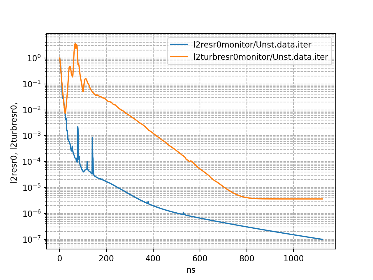
Continuity equation residual drops by 8 orders of magnitude within less than 1500 iterations while the SA model residual drop stalls after 3 orders of magnitude reduction.
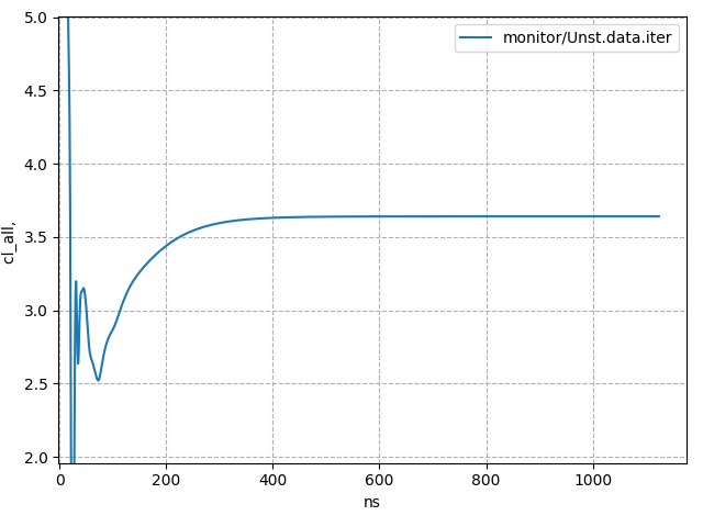
To verify force/moment convergence, you can plot the iterative history of the lift coefficient with:
References
NASA Langley Research Center, "2D Multielement Airfoil - Turbulence Modeling Resource," Available: https://turbmodels.larc.nasa.gov/multielementverif.html