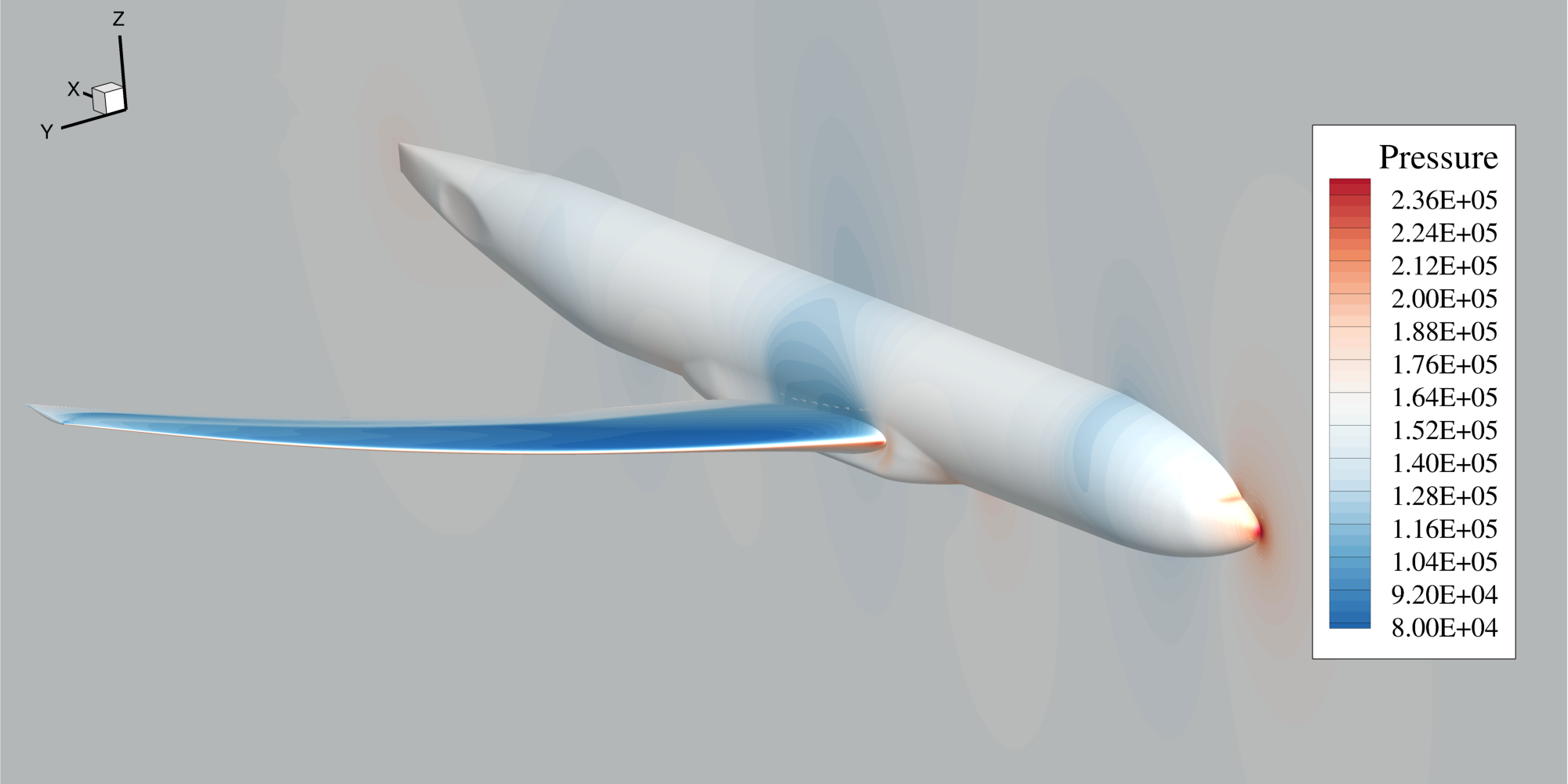
Aerodynamic Analysis using pyLAVA
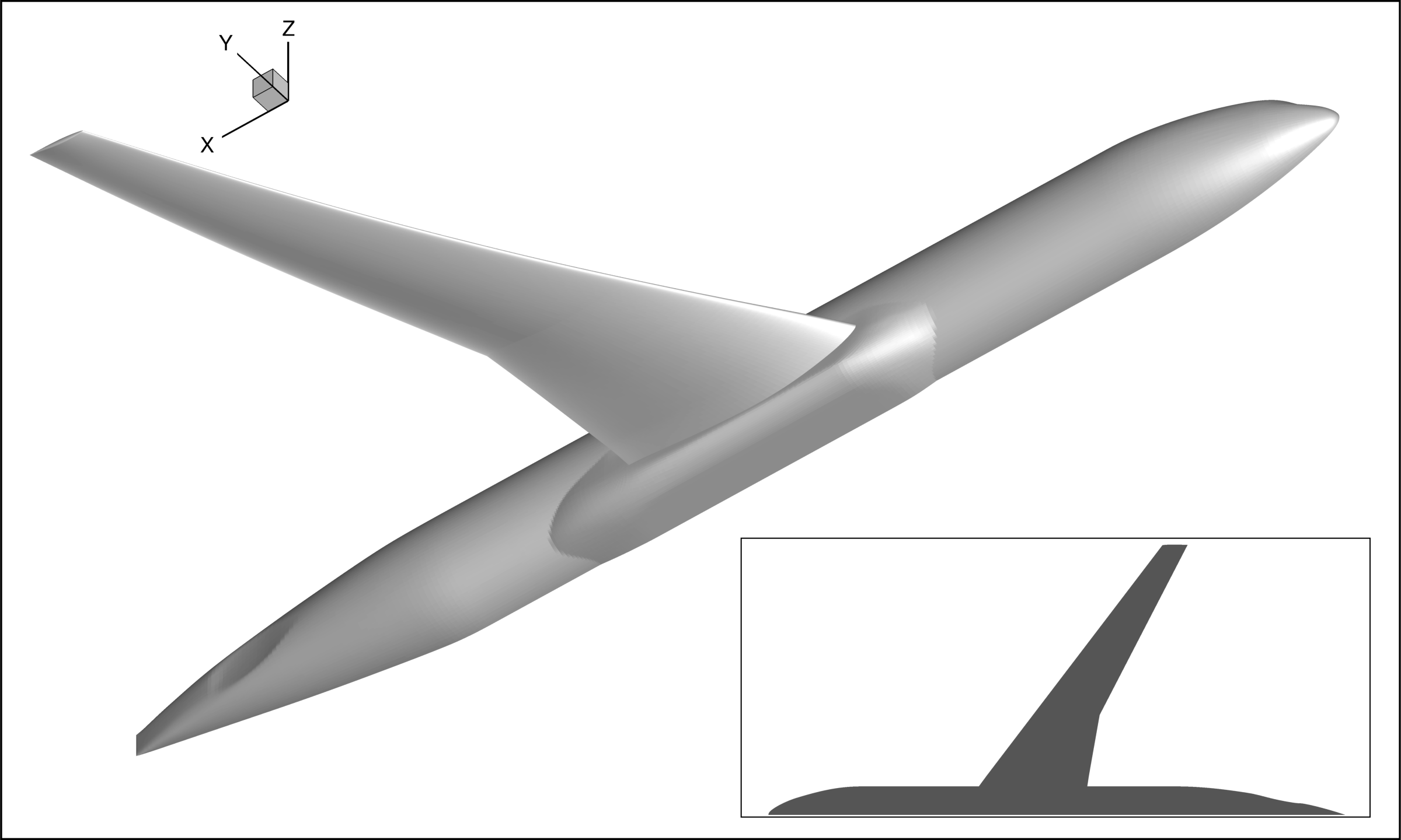
The goal of this tutorial is to replicate the aerodynamic analysis performed in the CRM Steady RANS tutorial using the Python interface to LAVA Curvilinear, pyLAVA. We will be demonstrating how to set up and run a flow solve using pyLAVA, as well as how to use some of the post-processing capabilities in pyLAVA to retrieve functionals and write solution files.
The LAVA class from the pyLAVA package is a python interface to the
LAVA Curvilinear framework. Some functionality that the LAVA class can perform includes, but is not limited to:
- initializing the flow solver
- perform a flow solve
- perform an adjoint solve
- write volume solutions
- deform the mesh
- evaluate user-specified functionals
- compute functional gradients
- so much more!
Prerequisites
Before starting this tutorial, ensure you have:
- LAVA solver installed and accessible — see LAVA Installation Guide
- Python 3.9 or above installed on your system
Environment Setup
For this example we will be using pyLAVA. See this documentation for information on setting up pyLAVA. This tutorial relies on Python packages listed in the Aerodynamic Analysis Requirements section.
We will be leveraging mpi4py in this tutorial, so I encourage you to include it in your Python environment.
However, if you are unable to use mpi4py on your system, you can still run this tutorial with a single MPI rank without mpi4py by remove the lines from mpi4py import MPI and comm=MPI.COMM_WORLD from the run_pylava.py script and running with a single MPI rank.
Tutorial Files
Make and navigate to a working directory of your choosing for this tutorial.
mkdir -p /path/to/lava_tutorials/crm_steady_rans_pylava
cd /path/to/lava_tutorials/crm_steady_rans_pylava
Download the input files for this tutorial:
| File | Description |
|---|---|
| grid.x.ihc | Grid file |
| grid.b2b | Block-to-block file |
| grid.bc | Boundary condition file |
| INTOUT | Interpolation and connectivity data |
| panel_weights.dat | Surface integration weights |
| run.yaml | LAVA solver input file |
| run_pylava.py | Python script for the analysis |
Arrange the downloaded files in the following structure:
crm_steady_rans_pylava/
├── run_pylava.py
├── run.yaml
├── grid.x.ihc
├── grid.b2b
├── grid.bc
├── INTOUT
└── overlapper/
    └── panel_weights.dat
Mesh setup
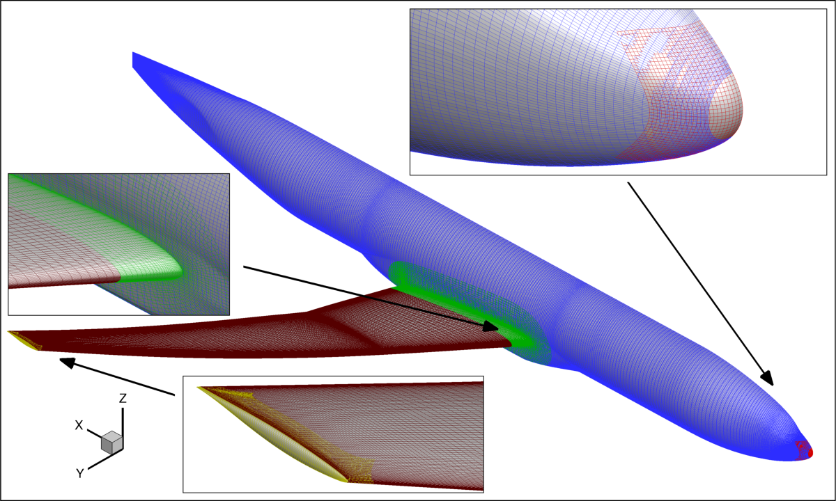
This tutorial uses the same grid as the one used in the CRM Steady RANS tutorial. The structured overset grid for the CRM wing body configuration consists of a main fuselage (blue), fuselage nose cap (red), wing/fuselage collar (green), main wing (maroon), wing outboard cap (gold), and octree based Cartesian off-body grid (black). The system consists of 5 near-body zones, 149 off-body Cartesian zones, and a total of 19,187,657 grid points. Boundary conditions for the grid system consist of no-slip walls for each l-direction = 1 near-body grid (assuming a j,k,l grid orientation), symmetry plane boundaries are specified for all surfaces on the y=0.0 plane, and far-field Riemann invariant boundary conditions are used for the outer-boundary of the Cartesian off-body grids. All non-specified boundaries are assumed to be either overset or block-2-block boundary conditions.
Solver Setup
The flow solver options are set using the run.yaml file.
The flow solver is run through the Python run script run_pylava.py.
Below, we break down the contents of these files.
Flow Solver Options
The run.yaml used in this tutorial file contains a standard set of options to run a RANS simulation in LAVA Curvilinear.
You can see all the flow solver options that you can define on this page.
Python Script
Now, let's break down the run_pylava.py script to understand how to use pyLAVA to run a flow solve.
Imports
Fairly straighforward, here we import thepylava and yaml packages.
Read YAML
Here, we have Python read the filerun.yaml. The returned object
lava_options is a dictionary containing all the options
that we will be using for LAVA.
💡 Tip: Modifying the options in Python
If you wanted to modify any options without changing the run.yaml file, you can do so after this line in the python script. An example may be if we were to add the line to modify the convergence tolerance to 1e-8 for the flow solver. However, any modification to the lava_options dictionary *after* the LAVA class is instantiated will have no impact on the flow solver options. All options are only passed to the flow solver when the LAVA class is first instantiated.Solver Instantiation
# Setup the aero solver instance
AeroSolver = LAVA(lava_options,
                  comm=MPI.COMM_WORLD,
                  suffix="3D.NS1.INTEL.AVX2.OPENMPI-lib")
Setting the suffix
When instantiating the LAVA Class, we have to tell it which LAVA dynamic library to use. This is done through the suffix argument.
The suffix is a string which is appended to the name of the LAVA dynamic library.
For example, if the suffix is INTEL.OMP, then the LAVA dynamic library that will be used is liblavacurv.INTEL.OMP.so.
You, the user, are responsible for setting the suffix to the correct value that corresponds to the compiled version of LAVA you want to use.
Solve
A direct call toAeroSolver() runs the flow solver!
Specifically, it makes a call
to the approximate-Newton-Krylov (ANK) solver in the lavacurv
framework. Thus, it solves the flow problem using the user-provided
options in the lava_options dictionary used to
instantiate the AeroSolver object.
Retrieving Functionals
# Evaluate some functionals
funcs = AeroSolver.evalFunction(['cl','cd'])

# Print the functionals to screen
if MPI.COMM_WORLD.rank == 0:
    print(f"C_L : {funcs['cl'][0]}")
    print(f"C_D : {funcs['cd'][0]}")
evalFunction function allows for the evaluation of a functional
of interest. Any surface-integration-based values (e.g. \(C_L\), \(C_D\)) can be obtained using this method.
These must be given to evalFunction as a list of strings.
A dictionary is returned which contains the resulting values for the functionals.
In this example, \(C_L\) can be retreived from the dictionary with the command
funcs['cl'].
Writing Volume Files
# Write out the volume file
AeroSolver.writeVolSolution(
   filename = "vol_pylava.q",
   filetype="plot3d",
   fields=["pressure", "velocityx", "velocityy", 'velocityz', "temperature", "nut"]
)
vol.q as a plot3d function file.
When it comes to writing surface files, pyLAVA uses a different capability compared to the normal LAVA executable.
Due to its roots in design analysis, pyLAVA leverages a "design surface", which must first be built before it can be used to write solution files. Design surfaces can be constructed from any collection of domain boundaries, probes, or immersed boundaries.
Writing Surface Files
# Write out the surface
AeroSolver.buildDVSurfaces(families=["fuse", "wing", "symm"])
AeroSolver.writeSurface(
   filename = "surface_pylava.plt",
   fields=["iblank", "pressure", "velocityx", "velocityy", 'velocityz', "temperature", "nut"]
)
fuse and wing families and the symmetry plane symm; these name were all originally specified in the grid.bc file as boundary condition families.
Currently, the writeSurface capability in LAVA only writes to Tecplot binary files.
Note
The family names given to buildDVSurfaces must match those given in the grid.bc file. If you are unsure of the family names, you can always open the grid.bc file and check.
Running
Running on the NAS Cluster
Aitken Supercomputer
First, modify the suffix argument in the run_pylava.py file to contain the following,
The following PBS script can be used to run this example on the NAS cluster using Aitken Rome Nodes.
job.pbs
#PBS -S /bin/bash
#PBS -N crm_rans_pylava_rom_curv
#PBS -l select=2:ncpus=128:mpiprocs=4:model=rom_ait
#PBS -l walltime=02:00:00
#PBS -j oe
#PBS -W group_list=<your project group ID>
#PBS -q normal

#BENCH reference crm_highspeed_curv.data.iter
#BENCH tolerance_abs 5.0e-4
#BENCH tolerance_rel 5.0e-4
#BENCH compare last_step
#BENCH exclude_vars stepl, d*, mind*, maxd*, flowres, turres, lin*, resturbulence1, resmomentum*, rescontinuity, resenergy
#BENCH save_vars cl_wing, cd_wing, cmy_wing

# Modules and Environments
module purge

# Load the module for LAVA
module use /swbuild/LAVA/LAVA_modules
module load LAVA

# Source the virtual environment which contains all
# the necessary python packages for optimization.
# The user is responsible for creating this virtual env
source path/to/virtual_env/bin/activate

# Set MPI environment variable
export MPI_NUM_MEMORY_REGIONS=0

cd $PBS_O_WORKDIR

# Run optimization script
log_file="run.log"
mpiexec -np 8 mbind.x -t 32 python run_pylava.py |& tee -a ${log_file}
Important
You must edit job.pbs before submitting this job, specifically:
- Replace
enter_group_idwith your actual group or project ID. - Replace
path/to/virtual_envwith the path to your Python virtual environment that contains the required Python packages.
mpi4py required for Aitken Supercomputer
We have found that when running on the Aitken Supercomputer, the line
must be the first line in therun_pylava.py script for the script to run properly.
If this line is not the first line, the Python command will stall.
Athena Supercomputer
First, modify the suffix argument in the run_pylava.py file to contain the following,
The following PBS script can be used to run this example on the NAS cluster using Athena Turin Nodes.
job.pbs
#PBS -S /bin/bash
#PBS -N crm_rans_pylava
#PBS -l select=1:ncpus=256:mpiprocs=4:model=tur_ath
#PBS -l walltime=02:00:00
#PBS -j oe
#PBS -W group_list=<your project group ID>
#PBS -q normal

cd $PBS_O_WORKDIR

# Modules and Environments
module purge

# Load the module for LAVA
module use /swbuild/LAVA/LAVA_modules
module load LAVA

# Source the virtual environment which contains all
# the necessary python packages for optimization.
# The user is responsible for creating this virtual env
source path/to/virtual_env/bin/activate

# Set environment variables for MPI and OMP
export MPI_NUM_MEMORY_REGIONS=0
export OMP_NUM_THREADS=64
export OMP_PLACES=cores
export OMP_PROC_BIND=close

#Solver
mpiexec -np 4 --ppn 4 --cpu-bind depth --depth 64 python run_pylava.py | tee run.out
Important
You must edit job.pbs before submitting this job, specifically:
- Replace
enter_group_idwith your actual group or project ID. - Replace
path/to/virtual_envwith the path to your Python virtual environment that contains the required Python packages.
Warning
At the time of writing, we have had difficulty using mpi4py across Turin nodes. Thus, you may currently only be capable of running this tutorial on a single Turin node.
Running on External Systems
Modify the suffix argument in the run_pylava.py file to match the suffix for the LAVA Dynamic Library that is compatible with your system.
Additionally, if the path to the LAVA Dynamic Library is not included in the LD_LIBRARY_PATH environment variable, then you will need to include the libPath argument when instantiating the LAVA class to specify the path to the LAVA Dynamic Library on your system. Together, these should look something like the following inside of your run_pylava.py file:
AeroSolver = LAVA(lava_options,
                  comm=MPI.COMM_WORLD,
                  suffix='lava_dynamic_library_suffix_for_your_system',
                  libPath='/path/to/lava/dynamic/library')
If you created a Python virtual environment following the directions in the environment setup instructions above, make sure to activate that environment in your terminal:
For a single MPI rank, you can run the following command,
For multiple MPI ranks, you can run the following command,
Proper Thread Binding for OpenMPI
When running with OpenMPI, proper thread binding may require additional flags for optimal performance. We have found that the following command ensures correct binding:
export OMP_NUM_THREADS=28
mpirun -np 4 --map-by slot:PE=$OMP_NUM_THREADS --bind-to hwthread python run_pylava.py | tee run.out
OMP_NUM_THREADS based on the number of threads you want to use.
Standard Output
During the preprocessing steps and flow solve, you will get the same screen output as from the executable. At the end of the output, you'll see the functionals written to screen,
Post-Processing
Thanks to the calls to writeVolSolution and writeSurface, we obtain a volume file vol_pylava.q and surface file surface_pylava.plt, respectively. The former is a plot3d function file which can be opened in conjunction with grid.x with any visualization software that handles plot3d format. The surface file is a Tecplot binary format.