QuickStart
This guide will take you through running the LAVACurv solver for a steady-state RANS
solution around an airfoil at transonic conditions.
Prerequisites
Before starting this tutorial, ensure you have:
- LAVA solver and utilities installed and your' environment properly setup, see LAVA Installation Guide
- Chimera Grid Tools (CGT) installed for optional mesh building
Tutorial Files
Download the input files for this tutorial:
| File | Description |
|---|---|
| grid.x | grid file |
| grid.bc | grid bc file |
| grid.b2b | grid block-to-block file |
| run.yaml | solver input file |
Obtaining the Grid
The easiest way is to download the grid directly from above, but alternatively you can generate a structured curvilinear grid. This section assumes you have Chimera Grid Tools (CGT) installed on your computer. First a structured curvilinear grid must be generated. In this case we download a grid from the AIAA Drag Prediction Workshop. Download the following zip file:
Once downloaded, unzip the directory and find the Plot3D grid file grid_OAT15A_Deck.x.
Now copy and past the following grided input file into a file named grided.inp located in
the same location as the Plot3D grid file:
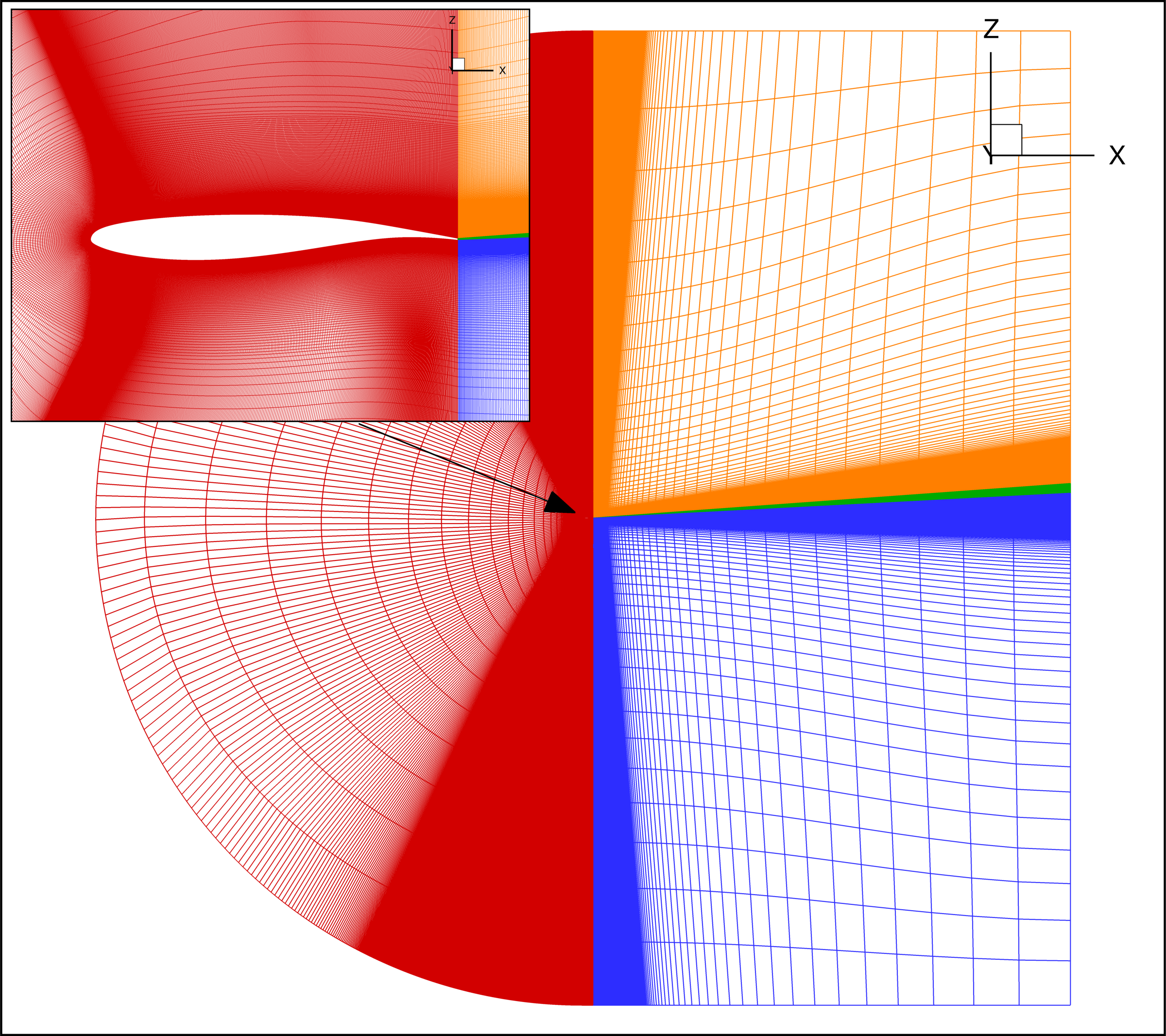
grid.x containing the ONERA OAT15A airfoil grid
generated by Sebastian Deck from ONERA1. This is a multi-block structured curvilinear
grid containing 4 zones: 1305x3x224, 160x3x224, 227x3x160, 160x3x224 for a total of
1200960 grid points. Here is an image of the grid system
 If you do not have CGT installed on your machine and want to use some
other grid generation software, then you will need to:
- rotate the grid by 90.0 degrees about the x-axis
- copy the 2D slice in both the positive y and negative y directions by 0.5
- concatenate the three 2D slices in the spanwise (y-axis) direction such that the first slice is at y = -0.5, the second slice is at y = 0.0, and the last slice is at y = 0.5
- swap indices between k and l (the 2nd and 3rd indices) such that k is in the span direction and l is in the wall normal direction
Setting up Boundary Conditions, Block-2-Block Conditions, and the Input File
Now that we have the grid, which is in meters, with a chord of 0.23 meters and a span of 1.0 meter, we can set up the boundary condition file.
At this point we simply need to associate a name for particular subsets of the grid. Below is the boundary condition file for this grid, grid.bc:
!       Name GridNumber   Jmin  Jmax  Kmin  Kmax  Lmin  Lmax
!*********** *********** ***** ***** ***** ***** ***** *****
        wall 1               1    -1     1    -1     1     1
         far 1               1    -1     1    -1    -1    -1
        symm 1               1    -1     1     1     1    -1
        symm 1               1    -1    -1    -1     1    -1
         far 2               1     1     1    -1     1    -1
         far 2               1    -1     1    -1    -1    -1
        symm 2               1    -1     1     1     1    -1
        symm 2               1    -1    -1    -1     1    -1
        wall 3               1    -1     1    -1     1     1
         far 3               1    -1     1    -1    -1    -1
        symm 3               1    -1     1     1     1    -1
        symm 3               1    -1    -1    -1     1    -1
         far 4              -1    -1     1    -1     1    -1
         far 4               1    -1     1    -1    -1    -1
        symm 4               1    -1     1     1     1    -1
        symm 4               1    -1    -1    -1     1    -1
With the boundary condition file complete, the block-2-block connectivity file can be generated with the following LAVA utility program command:
This will generate the followinggrid.b2b file:
!----------------------------------------------------------------------------------------------------------------------------
! BlkID     js     je        ks     ke        ls     le   DonorID    djs    dje       dks    dke       dls    dle    tx ty tz
!----------------------------------------------------------------------------------------------------------------------------
      1      1      1         1     -1         1     -1         2     -1     -1         1     -1         1     -1     1  2  3
      1     -1     -1         1     -1         1     -1         4      1      1         1     -1         1     -1     1  2  3
      2     -1     -1         1     -1         1     -1         1      1      1         1     -1         1     -1     1  2  3
      2      1     -1         1     -1         1      1         3     -1     -1         1     -1        -1      1    -3  2  1
      3      1      1         1     -1         1     -1         4      1     -1         1     -1         1      1    -3  2  1
      3     -1     -1         1     -1         1     -1         2     -1      1         1     -1         1      1     3  2 -1
      4      1      1         1     -1         1     -1         1     -1     -1         1     -1         1     -1     1  2  3
      4      1     -1         1     -1         1      1         3      1      1         1     -1         1     -1     3  2 -1
The final preprocessing step is to create an input yaml file for running the solver. Details of the inputs can be found at
Curvilinear User Guide-YAML Input File. For brevity we simply ask you to save the run.yaml file from the tutorial files section.
Running LAVACurv
With grid.x, grid.bc, grid.b2b, and run.yaml as input files we are ready to perform
steady-state RANS analysis on the ONERA OAT15A airfoil. Here we walk through setting up an example
PBS script to run on the NASA Advanced Supercomputing (NAS) computer using a Sky Electra node.
The commands are similar no matter where you decide to run this example.
The first step is to copy the aforementioned files into a working directory on Pleiades.
Next create a PBS file named run_sky.pbs with the following contents (note this is for c-shell users, see
Setup and Utilities for other options):
#PBS -S /bin/bash
#PBS -N oat_rans_curv
#PBS -l select=1:ncpus=40:mpiprocs=2:model=sky_ele
#PBS -l walltime=2:00:00
#PBS -q normal
#PBS -l site=needed=/home6+/nobackupp27
#PBS -j oe
#PBS -W group_list=<your project group ID>

#BENCH reference oat_rans_curv.data.iter
#BENCH tolerance_abs 1.0e-6
#BENCH tolerance_rel 1.0e-6

log_file="run.log"

module purge
module use /swbuild/LAVA/LAVA_modules
module load LAVA

unset F_UFMTENDIAN

cd $PBS_O_WORKDIR

mpiexec -npernode 2 mbind.x -t 20 lavacurv.3D.NS1.AVX2 run.yaml |& tee -a ${log_file}
run.out. An example of what your run.out file should look like upon completion can be downloaded below
Checking the Run
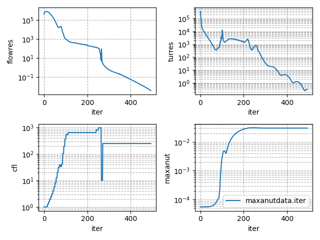
In order to plot the residual convergence history, use the plotHist.py python command
The convergence history of the integrated forces and momements along with the maximum Mach number in the domain can be plotted by
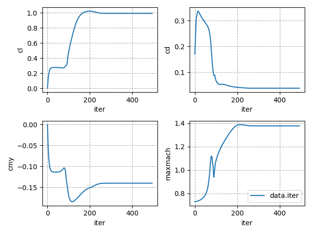
Here we see that the flow solver converged the L2 norm of the flow residual by the requested 8-orders of
magnitude yielding a lift coefficient of 9.914e-01, drag coefficient of 3.8800e-02, pitching moment coefficient
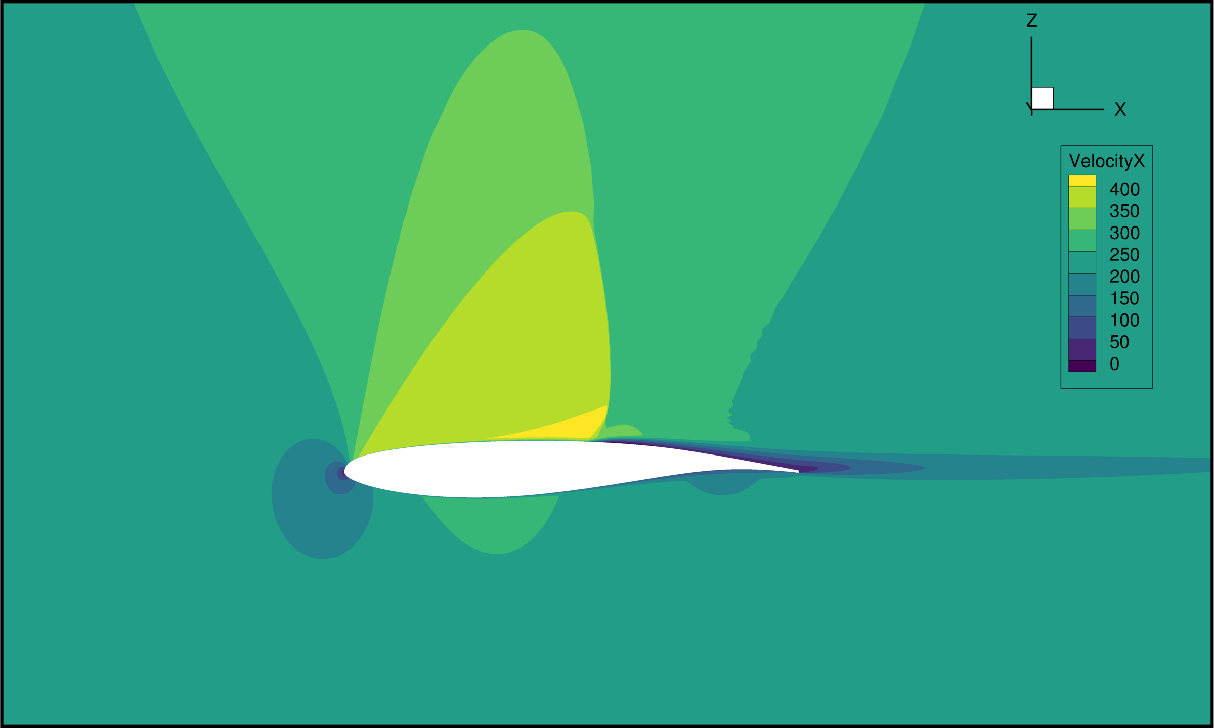
of -1.401e-01, and maximum Mach number of 1.377e+00. A plot of the x-direction velocity on a cutting
plane at y=0 is shown below.
You should now have a very basic understanding of how to use the LAVACurv flow solver and are ready to move on
in the documentation :)
Relevant Publications
-
Deck, S., and Renard, N., "Towards an Enhanced Protection of Attached Boundary Layers in Hybrid RANS/LES Methods," Journal of Computational Physics, Vol. 400, 2020, p. 108970. https://doi.org/10.1016/j.jcp.2019.108970 ↩