Voronoi Mesh Generator

The LAVA Voronoi mesh generation software creates polyhedral-cell tessellations for two- and three-dimensional computational domains. It also supports the subtraction of complex geometries through a clipping process, enabling the generation of body-fitted unstructured meshes. The mesher is designed for both shared and distributed memory parallelism.

The software is centered on the concept of the Voronoi cell. Given a collection of seeds \(\{{\bf s}_1,{\bf s}_2,\dots,{\bf s}_n\}\subseteq{\mathbb R}^d\), a \(d\)-dimensional Voronoi cell \(V_k\) is a subset of \({\mathbb R}^d\) of the form \(V_k = \{{\bf x}\in{\mathbb R}^d \ :\ {\rm for\ every}\ j\neq k,\ \|{\bf x}-{\bf s}_k\|_2\leq \|{\bf x}-{\bf s}_j\|_2\}\). In other words, \(V_k\) is a convex polyhedral cell which encompasses the region where points are closer to its generating seed \(s_k\) than any other seed in the domain.

Voronoi meshes have intrinsic properties that make them desirable for solving discretized governing equations. For example, faces are orthogonal to the vector connecting the two generating seeds on either side of the face and are also located midway between the seed points on either side. For a detailed presentation of the Voronoi tessellation properties and the current mesher's algorithms, see Sousa et al.¹.

Installation

Please refer to LAVA Voronoi Installation Guide for detailed instructions on acquiring and installing the Voronoi mesher.

Voronoi Mesher Inputs

Voronoi mesher uses a text-based input file in yaml format. In addition, geometry definition is provided to the mesher as a discrete triangulation.

Global parameters

We define the spacing between seeds in each refinement region relative to a reference length scale. This approach enables control of the overall mesh resolution and density through a single parameter. Once the user is satisfied with the point distribution at a given mesh density, generating coarser or finer meshes for a consistent refinement study becomes straightforward—simply adjust the reference length scale. For example, to use a reference length of 0.125, include the following in your input file:

reference_length: 0.125

Tip

If one sets the finest refinement region relative spacing to 1, then the reference length specified here will correspond to the length scale of the smallest cells, excluding potentially split cells, in the final mesh.

The Voronoi mesher can generate either a 2D Voronoi mesh with a single layer of cells or a fully 3D Voronoi mesh. In 3D mode, if the seed spacing in a given refinement region exceeds the thickness of the computational domain in one direction, only a single seed is placed at the domain's center along that axis. To toggle between 2D and 3D meshing, use the 2d input parameter. Moreover, the user can choose if the domain thickness in the \(z\)-axis is to remain with the prescribed z-extent (computational domain is defined as cube region) or if it will be made unitary by using the unitaryZmesh input. This parameter is only relevant when 2D mode is active.

#set to false for a 3d mesh.
2d: false 

#controls dimensionality of domain width in 2D mode.
unitaryZmesh: true 

Note

2D meshes are currently hardcoded to be aligned with the \(z\)-axis. If the user wants to build a 2D mesh of an airfoil, for example, the triangulation describing the surface shape needs to be aligned with the \(z\)-direction. The final mesh can be transformed, i.e. rotated, translated or scaled, before running the simulation in the unstructured solver.

Generating fully three-dimensional meshes can be computationally expensive. During the mesh design phase, users often need to iterate on refinement region layouts and seed densities. To streamline this process, the tool includes a 2d_plane_output option. This feature allows users to define an arbitrary plane, restrict seeding to a single cell layer normal to that plane, and produce a surface mesh that approximates a slice through the full 3D mesh. Additionally, this option can be used to generate planar triangulations whose density reflects that of the final mesh. These triangulations can be used for sampling the solution when running the unstructured solver. This cross sectional mesh tool is controlled by the following input section:

2d_plane_output:
  - active: true
    triangulate: true
    normalVector: [0, 1, 0]
    pointInPlane: [0,0.5,0]

Here, the active parameter controls whether the tool is enabled or disabled. The triangulate parameter controls the output format, if it is active, the generic Voronoi polygons will be triangulated and the final output will be composed of triangles only. In the case it is inactive, the output will consist of generic polygons that will approximate the slicing of a full 3D mesh by the chosen plane. Finally, the plane can be specified by the normalVector and pointInPlane parameters.

Finally, the user can control whether they wish to treat any of the coordinate directions as periodic with the periodicDir parameter. The entries correspond to the \(x\), \(y\), and \(z\) axes, respectively. When a direction is set to true, seeds near the boundary in that direction are mirrored across the opposite boundary as ghost-seeds during the graph-generation step, ensuring seamless periodic connectivity at the domain edges.

periodicDir: [false, false, false]

Note

The LAVA Unstructured solver has a flag (do lava voro periodic) that needs to be active to correctly account for the periodicity when a mesh built under these circumstances is used in a simulation.

Point cloud parameters

The Voronoi mesher can either generate a new point cloud from scratch based on refinement regions defined in the input file, or it can initialize the Voronoi graph from an existing set of points provided by the user. When a point cloud is loaded from a file, the seeding process is bypassed. This behavior is controlled using the following parameter:

# if reading point cloud from a *.csv file or *.bin specify true
read_points_from_file: false

If read_points_from_file is set to true, then the mesher loads the filename contained in the following parameter:

point_cloud_file: smoothed_final.csv

If read_points_from_file is set to false, the mesher performs seeding and writes two point cloud files to disk.

• unsmoothed.csv: Exported immediately after seeding, before point metadata is added and before Lloyd smoothing is applied.
• smoothed_final.csv: Written after metadata has been added and Lloyd iterations have smoothed the point distribution.

The output files can be saved in either binary or csv format, depending on user preference. The file type is controlled using the following setting:

# Specify as csv or bin
point_cloud_export_type: csv

Part of the process of generating the point cloud data structure involves labeling points with various metadata. These are related to identifying points close to the geometry in the case where the user has included a wall region and to identifying points to be smoothed. The information contained in this metadata is necessary for the correct usage of the Voronoi mesher but, if the user wants to restart the mesher from a point cloud file where this information has already been computed, for example, smoothed_final.csv, then they can skip this process by setting do_pointCloud_labeling to false:

# User may specify false if a previously labeled smoothed point cloud is used.
do_pointCloud_labeling: false

Initially, the volume transition between refinement regions of different cell spacing is abrupt. This volume jump can be smoothed by performing iterations of the Lloyd algorithm for generating centroidal Voronoi cells. To control the number of iterations, use the following input option.

# total number of lloyd iterations
lloyd_iter: 10

Note

In the applications we have attempted so far, 10 iterations seem to be enough to get a gradual volume transition between regions. A more extensive study on the influence of the number of Lloyd iterations still needs to be performed.

Following are some optional parameters for the case when the user would want to generate near-wall anisotropic meshes. For detailed usage with wall refinements, see the anisotropic near-wall spacing section.

Warning

Anisotropic meshing capability is currently under development and should be considered preliminary.

# User may specify either isotropic (default) or anisotropic.
near_wall_cell_type: anisotropic

# The number of surface smoothing iterations after curved surfaces
# are deemed sufficiently discretized
num_wall_pnt_lloyd_iters: 2

# Largest allowable angle between two anisotropic seeding rays.
# If angle is larger than that then the space between these rays
# is populated with extra anisotropic seeds at `max_ray_angle` intervals
max_ray_angle: 10

The algorithm behind the anisotropic seeding of the LAVA Voronoi mesher relies on first building a Voronoi diagram restricted to the surface of the geometry in question, then using this surface representation as a basis for near-wall anisotropic seeding. For this, the centroid and normal information of each face on the surface is used to create an anisotropic ray of seeds with a certain initial spacing and growth rate (discussed in the anisotropic near-wall spacing section). Locations where the geometry has discontinuities bigger than max_ray_angle are detected and a fan of rays at max_ray_angle intervals is seeded with the discontinuity at its origin. The anisotropic rays grow until the underlying Voronoi cells are isotropic and the remaining computational domain is seeded in an isotropic fashion. For this approach to work, a minimum discretization level is required at curved features of the geometry. These features are automatically detected and refined prior to the extra surface smoothing iterations indicated in num_wall_pnt_lloyd_iters being conducted.

Distributed memory parallelism parameters

The current implementation of distributed memory parallelism leverages the Voronoi tessellation capabilities of the mesher itself. A separate, superseding, Voronoi tessellation with one cell per MPI rank is used to separate the computational domain into geometrically defined regions which contain approximately the same number of cells in each of them. Load-balancing in terms of the number of cells is achieved by using an algorithm inspired by Fu et al. ², where an update for the seed of the load-balancing diagram is found by blending two procedures: the Centroidal Voronoi Tessellation (CVT) and the Voronoi Particle (VP) dynamics. In order to set this blending ratio and a threshold for what mean deviation from perfect balance is acceptable, use the following inputs:

#convergence criterion for load balancing
load_balancing_rms_threshold: 0.05
#blending between CVT and VP algorithms in load balancing
load_balancing_blending: 0.8
#max number of iterations in load balancing if convergence is not met
load_balancing_max_iter: 2000

The load_balancing_blending parameter controls the blend between VP and CVT methods, with valid values ranging from 0 to 1. A value of 0.8 means 80% VP and 20% CVT. The load_balancing_rms_threshold represents the acceptable RMS deviation from perfect load balance, expressed as a fraction (e.g., 0.05 = 5% deviation).

Note

The values shown here are default values that have been successfully used in various cases. Users should not need to modify these parameters under normal circumstances.

Since the Voronoi graph is fully defined by the location of the seed generating points, the partition can be saved in the same way as a point cloud file was. The inputs related to loading a previously defined partition are shown hereafter:

#specify true if user wants to restart from a previously defined partition.
read_partition_from_file: true
#partition point cloud file name
partitionPCfile: partitionPC.csv

Expert

There are additional parameters intended for advanced users or developers:face_connectivity_check, recompute_local_graph_every and dist_coeff. The face_connectivity_check option enables a debugging feature that verifies whether every non-wall cell face is correctly associated with a neighboring cell. This check helps catch issues where global connectivity may be lost in the locally generated graphs on each rank. The recompute_local_graph_every parameter is used to speed up the parallel Lloyd smoothing process by skipping the update of ghost seeds at every iteration. While this may lead to slight differences in the final smoothed point cloud compared to a single-rank run, the deviations are generally minimal due to the small incremental movements of seeds during each iteration. Lastly, the dist_coeff parameter expands the ghost cell buffer around each partition. This is used to ensure the proper global connectivity information is retained for split ghost cells. These parameters are specified in yaml format as shown below:

#specify true if user wants to check if all faces have neighbors.
face_connectivity_check: false

#do lloyd smoothing without recomputing true local graph for N iterations, then recompute it
recompute_local_graph_every: 1

#distance multiplier when trying to find ghost cells.
#value needs to be >= 1.
dist_coeff: 1.5

Refinement regions parameters

Because a Voronoi tessellation is fully described by the distribution of points inside the domain of interest, the task of generating a high-quality mesh is simplified to placing seeds strategically and in a somewhat automated fashion. The process begins by defining the computational domain that bounds the Voronoi tessellation, followed by populating it with refinement regions. Each region is assigned a characteristic length scale that determines the base spacing between seed points. This length scale is inversely proportional to the number of cells in each region. Refinement regions can overlap and, when that occurs, the region with the smallest length scale is given priority.

The following region types are supported in the current Voronoi mesher:

cube

    - name: rectangular_prism_example
      type: cube
      seed: bodycentered
      smoothing_layers: 3
      spacing_rel: [4, 4, 4]
      distance: [10.0, 5.0, 7.5]
      center: [0.0, 0.0, 0.0]
      angles: [0.0, 0.0, 0.0]
      telescoping_refinement:
        - spacing_growth: 2
          num_points_per_layer: 8
          max_spacing_rel: 100

Each region has a name that will be used to identify it in the log file. The name parameter is arbitrary. The type parameter is used to distinguish the region's category. In this case, its type is a cube. The initial seeding is done in lattices and it is controlled by the seed parameter. The valid options for seeding patterns are cartesian, bodycentered, facecentered, or hexprism.

The choice of seeding pattern determines the resulting Voronoi cell shapes:

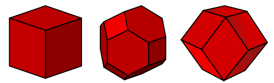
• cartesian: Produces cubic cells (regular hexahedra) (left)
• bodycentered: Body-centered-cubic (BCC) lattice, produces truncated octahedra (middle)
• facecentered: Face-centered-cubic (FCC) lattice, produces rhombic dodecahedra (right)
• hexprism: Produces hexagonal prisms

Every region optionally has smoothing_layers. This defines the number of seed layers, starting from the boundary between regions, that will be targeted for Lloyd smoothing.

The spacing between neighboring seeds in the lattice is determined by multiplying spacing_rel in the corresponding coordinate axes with reference_length input number. Alternatively, the user may specify an absolute spacing value by using spacing_abs instead. This is not encouraged since it decouples the region from the reference_length parameter and makes it harder to conduct consistent mesh refinement studies.

Warning

Despite the input supporting different seed spacing in the different axial directions, the mesher has only been tested with isotropic seeding at this point. Therefore the spacing entries for each axis should be the same currently.

The distance parameter controls how the three \((x_1,x_2,x_3)\) axes of the bounding cube are scaled into a general rectangular prism in absolute values. The vector center determines the center point of the box. The angles parameter controls the rotation, in degrees, of the region relative to its own coordinate axes.

Note

A refinement region of type: cube is volumetric, i.e. it defines a region of space where all the seeds inside this region will have the same spacing.

Finally, the telescoping_refinement input section allows the user to smoothly transition the refinement region into the freestream. If this section is provided, the mesher will generate a series of layers, each with a thickness corresponding to a user-defined number of cells, set by the num_points_per_layer parameter. In each successive layer, the seed spacing increases according to the spacing_growth factor. This process continues until the seed spacing reaches the user-specified max_spacing_rel value. Alternatively, a max_spacing_abs can be provided also.

Warning

The max_spacing_rel may not exceed the spacing of the freestream value used when specifying the computational domain bounding box.

ellipsoid

The type: ellipsoid region can be used to define either spherical or ellipsoidal volumes, within which seeds are placed using a user-defined spacing. The distance parameter is used to scale the axes of a sphere into an axis-aligned ellipsoid. If the same value is used for the 3 entries, then it is a sphere and the value is its radius.

  - name: ellipsoid_example
    type: ellipsoid
    seed: bodycentered
    smoothing_layers: 3
    spacing_rel: [8, 8, 8]
    distance: [2, 2, 2]
    center: [1.0, 2.0, 3.0]
    angles: [0.0, 0.0, 0.0]
    telescoping_refinement:
      - spacing_growth: 2
        num_points_per_layer: 8
        max_spacing_rel: 100

All the other parameters in this region input block have the same use and meaning as previously described in cube.

frustum

In order to specify a cylinder, cone, or frustum shaped seeding region, use the frustum region type.

  - name: frustum_example
    type: frustum
    seed: bodycentered
    smoothing_layers: 2
    axis_start: [1, 0, 2]
    axis_end: [-1, 0, -2]
    radius_start: 0.75
    radius_end: 0.5
    inner_radius_start: 0.5
    inner_radius_end: 0.25
    spacing_rel: [1, 1, 1]
    telescoping_refinement:
      - spacing_growth: 2
        num_points_per_layer: 8
        max_spacing_rel: 100

Many of the options for the frustum region are similar to those used for the cube or ellipsoid types. A frustum is defined by a central axis, which starts at axis_start and ends at axis_end. These points determine both the direction and the length of the frustum along its axis. The shape is formed by two circular faces, each perpendicular to this axis. The radius of the circle at axis_start is given by radius_start, and the radius at axis_end is specified by radius_end—both provided as absolute values. If the two radii are equal, the shape becomes a cylinder. Additionally, the frustum can be made hollow by specifying inner radii using inner_radius_start and inner_radius_end.

telescoping_frustum

In jet noise prediction simulations, we have observed that abrupt changes in cell volume near the shear layer can impact far-field noise predictions. We also identified an opportunity to gradually increase cell size with distance from the jet source to reduce computational cost without compromising accuracy. To support this, we developed a specialized region type—telescoping_frustum—which provides finer control over cell volume transitions along a user-defined frustum axis. This region allows the user to specify a spacing_growth factor and control layer thickness through the num_points_per_layer parameter.

In standard regions, seed lattices are aligned with a global origin, enabling seamless overlap between regions that share the same spacing. However, this can lead to slight inconsistencies in spacing at region boundaries. The telescoping_frustum is the only region type where the seeding lattice is not aligned to the global axis. Instead, its layer origins are carefully positioned to maintain consistent spacing across region boundaries.

Additionally, this region type includes an option for radial_refinement, allowing for a smooth transition between the refined volume and the freestream spacing of the surrounding computational domain. It works on the same principle as the telescoping_refinement section present in previous region type definitions, using spacing_growth, num_points_per_layer, and max_spacing_rel (or max_spacing_abs) parameters to control the gradual transition in cell size.

  - name: telescoping_frustum_example
    type: telescoping_frustum
    seed: bodycentered
    smoothing_layers: 2
    frustum:
      - axis_start: [0.7, 0.0, 0.0]
        axis_end  : [1.75, 0.0, 0.0]
        radius_start: 0.75
        radius_end  : 0.95
        inner_radius_start: 0.25
        inner_radius_end  : 0.11
        spacing_start_rel: [1, 1, 1]
        spacing_end_rel: [4, 4, 4]
        spacing_growth: 1.2
        num_points_per_layer: 25
    radial_refinement:
      - spacing_growth: 2
        num_points_per_layer: 5
        max_spacing_rel: 100

wall

A type: wall region allows the user to introduce a geometric surface into the mesh. This surface is imported as a triangulation via the trifile parameter, with support for three file formats: *.fro, *.cgns and *.i.tri. The triangulation must meet two key requirements: it must be watertight (i.e., fully closed), and all surface normals should be consistently oriented in the same direction. The triangulation included here will be used as clipping surface and its boundaries will be included in the final mesh definition.

Note

Many meshers require input triangulations where triangle sizes are on the same order of magnitude as the final mesh cells. In contrast, the current Voronoi mesher only needs an accurate representation of the geometry’s curved features. Flat regions, for instance, can be captured using just two triangles without any loss of accuracy.

Note

The LAVA Voronoi mesher supports multiple instances of the wall region. However, whenever possible, it is recommended to use a single closed triangulation that defines the full geometry of interest. Unnecessary intersecting surfaces increase computational overhead and can lead to clipping failures in edge cases not yet addressed by the LAVA team. At present, multiple triangulations are primarily recommended for cases involving sliding interfaces, where separate meshes are required for the static and rotating components.

Here is an example of an input block for a wall region:

- name: wall_region_example
  type: wall
  trifile: triangulation_example.cgns
  smoothing_layers: 4 #Controls Lloyd smoothing of seed layers adjacent to the wall geometry
  project_layers: 2
  seed_toward_normal: true
  directional_seeding: false
  face_merge_angle : 30
  #---start expert inputs---#
  angle_exceptions:
    - face_merge_angle: 5
      components: 3, 4
    - face_merge_angle: 15
      components: 5
  check_subcomponents: false
  tangential_plane_pert_factor: 0.01
  do_triangulation_checks: true
  do_export_gap_triangles: false
  #----end expert inputs----#
  #---start optional inputs---#
  rotate:
      - center: [0.0, 0.0, 0.0]
        axis: [0, 0, 1]
        angle: 45.0
  translate: [1.0, 0.0, 0.0]
  #---end optional inputs---#
  refinements:
    - name: example_ref_1
      seed: bodycentered
      smoothing_layers: 2 #Controls Lloyd smoothing at boundaries between refinement levels
      level_points_per_thickness: 8
      level_spacing_inner_rel: 2
      level_spacing_outer_rel: 100
      level_spacing_growth_rate: 2
      components: 3-5
      #----start optional anisotropic inputs----#
      initial_wall_normal_spacing_rel: 0.01
      wall_normal_spacing_growth_rate: 1.2
      #----end optional anisotropic inputs----#
      #---start expert inputs---#
      remove_1st_wall_layer_extra_points: true
      #---end expert inputs---#
    - name: example_ref_2
      seed: bodycentered
      smoothing_layers: 2
      num_levels: 2
      level_spacings_rel: [1, 2]
      level_thicknesses: [0.25, 0.25]
      components: 2

There are five key parameters associated with a wall region that casual users should understand: smoothing_layers, project_layers, seed_toward_normal, directional_seeding, and face_merge_angle.

• smoothing_layers: Determines how many layers of seeds near the geometry will be smoothed using the Lloyd iteration process.
• project_layers: Specifies how many layers of seeds will be adjusted in the wall-normal direction to ensure their spacing remains consistent with the region’s target seed spacing.
• seed_toward_normal: Defines which side of the triangulation represents the fluid domain and which represents the solid. This controls where seeds are added or removed and dictates which portions of the mesh are clipped away during the geometry subtraction phase.
• directional_seeding: Determines whether wall-distance-based refinement regions should expand in all directions regardless of surface normal orientation, or only if the direction pointed to by the surface normal should be taken into account. If directional_seeding is set to true then only the direction that points towards the fluid domain, given in combination of the surface normal orientation and the seed_toward_normal parameter, is considered valid for in region tests.
• face_merge_angle: Sets a threshold, in degrees, for merging neighboring triangles based on the similarity of their normals. Triangles with normal vectors within this angular threshold are treated as part of the same smooth surface and will be merged during the clipping process. This classification is performed on a component-by-component basis. Therefore, if the loaded triangulation is already divided into different regions, these divisions will be preserved in the final mesh.

Expert

Expert users have extra parameters that could be added to a wall region definition. These are the angle_exceptions input section, the check_subcomponents parameter, the tangential_plane_pert_factor, do_triangulation_checks, and do_export_gap_triangles.

• angle_exceptions: This input section enables the user to apply different face merge angle criteria to different components. For instance, in an iced wing application, the user may wish to use distinct criteria for the iced region compared to the smooth areas of the wing. Multiple exceptions can be added within this section, with each entry consisting of its own face_merge_angle and a list of components to which this angle threshold applies.
• check_subcomponents: In rough triangulations, such as those for accreted ice, the algorithm used to classify smooth regions (referred to as subcomponents) may create a subcomponent where two triangles share only a single vertex. This situation can cause issues for the clipper algorithm. The check_subcomponents parameter determines whether an additional check is performed during the classification step to identify and handle this single-vertex triangle neighbor case.
• tangential_plane_pert_factor: The projection step might create equidistant seeding patterns that may lead to degenerate cases during the Voronoi seed generation. A tangential random perturbation of the projected layers is performed to remove degeneracies. The tangential_plane_pert_factor defines the maximum magnitude of this perturbation as a fraction of the local seed spacing.
• do_triangulation_checks: When the mesher reads a triangulated surface, it automatically performs a suite of integrity checks—verifying that the surface is watertight, consistently oriented, and free of degenerate connectivity—and attempts to correct any orientation inconsistencies it finds. This behavior is controlled by do_triangulation_checks (default true). Disabling it skips the checks and simply populates the triangle neighbor data structure, which can be useful to reduce startup time when the triangulation is already known to be valid. As part of these checks, the mesher also verifies that the wall-normal gap available between facing surfaces is larger than the first-layer wall-normal spacing for each component, emitting a warning if any component fails.
• do_export_gap_triangles: A debug companion to the gap check described above (default false). When set to true, the mesher writes one OBJ file per offending component containing the source triangle, the opposing hit triangle, and a line segment connecting their centroids at the measured gap distance. These files can be loaded in a visualization tool to quickly locate and fix the problematic region of the triangulation.

Casual users should not add these entries to their input file. Their default values should be valid for most cases.

Optional

• rotate and translate: These allow the user to apply a rigid body transformation to the loaded triangulation before it is used. rotate takes a sub-section with center (3-element array), axis (3-element array), and angle (scalar, in degrees). translate takes a 3-element array [dx, dy, dz]. At most one instance of each is currently supported. When both are specified, the rotation is always applied first, followed by the translation.

Each wall region has a refinements input section. The refinements section is responsible for introducing seeding regions based on the distance to the triangulation introduced in trifile in the computational domain. This section is composed of blocks of two types that have shared and specific parameters. In the previously added wall example block there are two refinement sections: example_ref_1 and example_ref_2. Both of them have the following common parameters: name, seed, smoothing_layers and components, which are defined hereafter:

• name: Arbitrary string used to identify the region in the logfile.
• seed: Seeding pattern. See cube region for a more thorough description.
• smoothing_layers: Determines how many layers of seeds between refinement region boundaries will be smoothed using the Lloyd iteration process.
• components: Determines which sections of the triangulation will be used as a basis for the distance calculation to determine the boundaries of each refinement region. Components may be added as numbers, "components: 1, 2, 3", as intervals, "components: 1-3" or by name, for example, "components: slat, main, flap".

Expert

Expert users have access to an additional parameter that can be added to the refinement section of the wall region: remove_1st_wall_layer_extra_points.

This parameter controls whether points marked as belonging to the first wall layer — and that only have neighbors also in the first wall layer — are removed from the point cloud. Under normal circumstances, removing these extra points is recommended. However, in regions where small gaps exist relative to the local seed spacing, there may not be room for other points to be assigned to additional wall layers, and unnecessary removals can occur. For example, this behavior was observed when meshing a wing with horn ice accretion and its value was set to false, turning off the default behavior.

Tip

If the user does not know the component numbers and/or names, they may run the mesher and stop execution after the triangulation is read and its contents are output to the screen or logfile. One example output is:

Reading triangulation from crmhl-2dcut.igs.cgns
CGNS lib  version : 4200
CGNS file version : 4
Done reading
Number of nodes      : 82190
Number of triangles  : 164368
Number of components : 4
.... PID: 1   name: slat
.... PID: 2   name: main
.... PID: 3   name: side
.... PID: 4   name: flap
Finished reading triangulation file:  crmhl-2dcut.igs.cgns

Anisotropic Near-Wall Spacing (Optional)

Optional

In the refinement section, the user has the option of specifying the wall-normal spacing in the near-wall region and its growth via the following parameters: initial_wall_normal_spacing_rel and wall_normal_spacing_growth_rate, respectively. Note that the value chosen for initial_wall_normal_spacing_rel must be smaller than the isotropic distance between seeds introduced in the level_spacing_inner_rel parameter. These values are only relevant if near_wall_cell_type is set to anisotropic in the Point cloud parameters section.

The parameters in the two types of refinement section blocks differ based on how they define distance-based seeding volumes.

In example_ref_1, a telescoping strategy is used. A sequence of nested regions is generated, each with a thickness determined by the number of points per layer, controlled by level_points_per_thickness. The refinement begins near the surface, using the initial spacing specified by level_spacing_inner_rel. As each subsequent layer is created, the local spacing increases by a factor defined by level_spacing_growth_rate. This process continues until the spacing reaches the value given in level_spacing_outer_rel.

Warning

The level_spacing_outer_rel may not exceed the spacing of the freestream value used when specifying the computational domain bounding box.

In contrast, example_ref_2 adopts a manual specification approach. It defines the number of refinement levels using num_levels, and explicitly provides the relative spacings and absolute thicknesses for each level via the level_spacings_rel and level_thicknesses parameters, respectively.

All seed spacing parameters that end with _rel are relative to the reference_length parameter discussed in the Global parameters section of this manual. If the user wants to introduce absolute spacing values, they may change the ending to _abs.

Tip

The telescoping strategy used in example_ref_1 is the LAVA group’s preferred approach for generating wall-modeled LES meshes. When this method is applied, globally refining the mesh by halving the reference_length results in approximately a fourfold increase in the total number of cells. In contrast, using the approach in example_ref_2 leads to about an eightfold increase under the same refinement. The increase is smaller in the first strategy because both the seed spacing and the layer thicknesses are reduced simultaneously.

If the user wants to specify a cylinder as a triangulated surface they do not need to provide the triangulation file for it. The user can simply define the parameter trifile as cylinder and define the cylinder via simple geometric and discretization parameters. The cylinder can be specified using either: (center, axis, height, radius) or (axis_begin, axis_end, radius). The angle_resolution parameter (in degrees) controls the circumferential discretization: smaller values create more triangles around the cylinder's perimeter for a smoother surface. A sample cylindrical wall region input is as follows:

  - name: cylinder_example
    type: wall
    seed_toward_normal: true
    trifile: cylinder
    geom_parameters:
      - center: [-0.256326208, -0.256326208, 0.053750000]
        axis: [0, 0, 1]
        radius: 0.2
        height: 0.025
        angle_resolution: 2
    isDomainBoundary: true
    smoothing_layers: 4
    project_layers: 2
    face_merge_angle: 5
    refinements:
      - name: cylinder_ref
        seed: bodycentered
        smoothing_layers: 3
        level_points_per_thickness: 4
        level_spacing_inner_rel: 16
        level_spacing_outer_rel: 1000
        level_spacing_growth_rate: 2
        sliding_interface_inner_spacing_auto_detection:
          - active: true
            rotating_region_names: blade1

A cylindrical surface can be used in two ways: either as a regular wall surface or as the surface defining the sliding interface between a rotating and a static domain. In the latter case (as in the previous example), two additional entries are important: the isDomainBoundary parameter and the sliding_interface_inner_spacing_auto_detection subsection.

• isDomainBoundary This parameter specifies whether the triangulation is part of a domain boundary. Its default value is false, but for a sliding interface it must be set to true.

• sliding_interface_inner_spacing_auto_detection This subsection can optionally be used to automatically detect the smallest rotating region spacing that reaches the sliding interface. When enabled, it adjusts the level_spacing_inner_rel to this detected value instead of the user-specified one.

  • To activate this feature, set the active parameter to true.
  • The rotating_region_names parameter must list all rotating regions inside the sliding interface that should be tested.
  • If multiple regions are present, list them consecutively and separate them with commas, e.g.:

  rotating_region_names: blade1_leading_edge, blade1_main_element, blade1_trailing_edge
  

Important

All listed regions must have been previously defined in the inputs.yml file.

tri

A type: tri region allows users to define arbitrary shapes using triangulated surfaces. These surfaces can serve as boundaries for volumetric refinement regions or as the basis for distance-based seeding. Unlike wall regions, multiple tri regions may be included and the triangulation files in them do not need to form watertight surfaces—provided the volumetric_seeding section is omitted. One common use case for an open triangulated surface is marking the approximate location of a shock, enabling targeted refinement based on distance.

Most parameters in a tri region mirror those of a wall region. The key distinction is the optional volumetric_seeding block, which is used when the user wants to fill the interior of a closed triangulated surface with a uniform seed spacing. This input block type may be omitted otherwise. Each volumetric_seeding section includes four parameters: name, seed, smoothing_layers, and spacing_rel, all of which have been described earlier in this manual.

An example input block for a tri region is included hereafter:

  - name: user_defined_tri_region_example
    type: tri
    seed_toward_normal: false
    trifile: other_triangulation_example.cgns
    refinements:
      - name: tri_dist_refinement_example
        seed: bodycentered
        smoothing_layers: 2
        level_points_per_thickness: 8
        level_spacing_inner_rel: 2
        level_spacing_outer_rel: 100
        level_spacing_growth_rate: 2
        components: 1
    volumetric_seeding: # if this section is included, triangulation must be closed.
      - name: user_def_volume_example
        seed: bodycentered
        smoothing_layers: 2
        spacing_rel: 1

Yaml input examples

In this section, examples of complete input files are included.

• Simple volumetric seeding
• Multielement airfoil
• OAT15a
• Round jet
• RANS Multielement airfoil
• Sliding interface example

Warning

If one inspects the files, they will note that the first entry in the region: input block is always an axis-aligned cube region. This is mandatory. The first region is what defines the computational domain's bounding box and the freestream refinement level.

Note

Example surface triangulation files are provided for the multielement airfoil and OAT15a cases. The simple volumetric seeding option does not require a triangulation. For the round jet case, a triangulation is not included; however, the roundjet.yml file is provided as an example of how to configure a telescoping_frustum region.

References

---

1. Sousa, V., Rodgers, A. K., Sriram, K., Sozer, E., Barad, M. F., Stich, G.-D., Cadieux, F., and Duensing, J., "LAVA Voronoi Mesher for Wall-Modeled Large-Eddy Simulations," American Institute of Aeronautics; Astronautics, July2024. https://doi.org/10.2514/6.2024-4306 ↩

2. Fu, L., Hu, X. Y., and Adams, N. A., "A Physics-Motivated Centroidal Voronoi Particle Domain Decomposition Method," Journal of Computational Physics, Vol. 335, 2017, pp. 718--735. https://doi.org/https://doi.org/10.1016/j.jcp.2017.01.051 ↩