Genesis Capsule WMLES

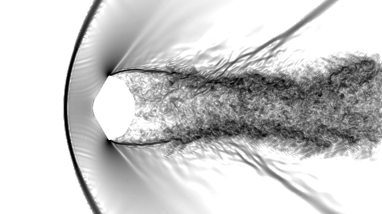
Density gradient magnitude contours in logarithmic scale

This tutorial outlines a Wall-Modelled Large Eddy Simulation (WMLES) setup of the Genesis sample return capsule as tested in the Aeroballistic Research Facility at Eglin AFB. The test details and results are summarized by Cheatwood et al.¹. Although ballistic test flight speed varies during the trajectory, the simulation is setup based on an average \(\textrm{Mach}=1.44\), \(\textrm{Re}=2.3\times10^6\) condition. Model geometry for the simulation is setup as full scale whereas the ballistic test was done with \(0.047\) scale model.

Prerequisites

Before starting this tutorial, ensure you have:

• LAVA solver installed and accessible — see LAVA Installation Guide
• LAVA Voronoi mesher installed — see Voronoi Installation Guide
• Basic familiarity with LAVA input file structure — see Unstructured Solver Inputs

Tutorial Files

Download the input files for this tutorial:

File	Description
genesis_capsule_surface_tri.cgns	Surface geometry triangulation
voro_genesis_capsule.yml	Voronoi meshing input file
unst_genesis_capsule.inputs	Solver input file
job_gh200.pbs	Sample PBS file for the solver run on NAS GH200 nodes

Directory Setup

Create a working directory for this tutorial with separate folders for meshing and simulation:

mkdir -p genesis_capsule/{meshing,run}
cd genesis_capsule

Place the downloaded files in the appropriate folders:

• voro_genesis_capsule.yml → meshing/
• genesis_capsule_surface_tri.cgns → meshing/
• unst_genesis_capsule.inputs → run/

If you are running on NASA's NAS systems, also place the PBS scripts:

• job_gh200.pbs → run/

Warning

Make sure to replace the #PBS -W group_list=<your project group ID> line with the correct group id you will use

Meshing

The Voronoi meshing input for the genesis capsule specifies a telescoping refinement zone emanating from the front shell and side surfaces as well a cylindrical wake refinement region extending 4 diameters downstream. Both zones gradually coarsen towards farfield which extend about 6D upstream, 16D in the transverse direction and 20D in the downstream direction.

To generate the mesh using the LAVA Voronoi generator, navigate to the meshing/ directory and generate the mesh:

cd meshing/
export OMP_NUM_THREADS=32
lavavoro.AVX2 ./voro_genesis_capsule.yml

Executable Names

The Voronoi executable name varies by architecture. See the Voronoi Installation Guide for details.

PBS Setup on NAS

If running on NAS systems, ensure that you have read the [Running On NAS Guide] (../../../setup_docs/lava_on_NAS.md) for example PBS setup scripts.

Note

The provided Voronoi input file will generate a coarser mesh than required for mesh insensitive results. You can reduce the reference_length parameter in the voro_genesis_capsule.yml for finer meshes.

This generates voro_genesis_capsule.cgns in the current directory. Link this file to the run directory:

cd ../run
ln -sf ../meshing/voro_genesis_capsule.cgns ./

Solver Inputs

The simulation is setup to integrate \(100\) CTUs (convective time units based on capsule diameters) using a \(3^\mathrm{rd}\) order accurate explicit time integration.

time {
  steady      = false
  finish ctu  = 100
  initial cfl = 0.05
  cfl         = 2.
}

unst {

  explicit {
    method = ssprk33
  }
}

Diagnostics section is setup to filter cells that are smaller than intended, up to a maximum of \(0.05\%\) of cells. These few cells apply a smoother to their solution field at every time step to avoid restricting the explicit time step size severely. The target size filter entry here corresponds to the smallest cell expected by Voronoi sizing regions, and it corresponds to the reference_length setting the in the provided voro_genesis_capsule.yml Voronoi input file.

  diagnostics {
    # Target size filter here is smaller than the actual smallest
    # cell size in the grid to avoid filtering any surface cells
    target size filter   = 0.007385
    max percent filtered = 0.05
  }

The KEEPBLEND scheme, which blends a kinetic energy preserving central flux and a MUSCL reconstructed upwind flux is utilized. The upwind blending is controlled by a Ducros type sensor, that can optionally be further localized with the enstrophy factor multiplier. In this case, the multiplier is unity which recovers the original Ducros formulation. add shock dissipation = true activates a sensor based addition of Rusanov flux near shocks only.

  convective terms {
    scheme = KEEPBLEND
    order = 2
    limiter = minmod
    flux function = ausmpw+
    add shock dissipation = true
    upwind blending sensors = [ducrosmod]
    upwind sensor enstrophy factor = 1
  }

Running the Simulation

Following example is for running on NAS's GH200 system. From pfe front-end, login to Cabeus Grace Hopper front end (cghfe01 or cghfe02) and submit the PBS script.

ssh cghfe01
cd path-to-your-case-directory/run/
qsub job_gh200.pbs

Note

Make sure to inspect and alter the provided pbs file for your system. If you are using NAS resources, make sure to set the group_list to correct value.

Output and Results

LAVA creates several subdirectories to organize the simulation output:

• volume/ - Volume solution files in CGNS format (Unst.vol.########.cgns)
• surface/ - Surface solution files and boundary condition statistics (Unst.surf.########.cgns, bc_stats_*.dat)
• restart/ - Restart files for continuing simulations (Unst_restart.########.hdf5)
• monitor/ - Time-stepping and iteration monitoring data (Unst.data.iter)
• isosurface/ - In-situ isosurface extractions (defined as span cut-planes for this case)

The volume files contain the complete flow field solution and can be visualized using tools such as ParaView or Tecplot. For convenience, LAVA creates symbolic links (Unst.volLatest.cgns, Unst.surfLatest.cgns) that always point to the most recent solution files.

Monitoring Force/Moment Convergence

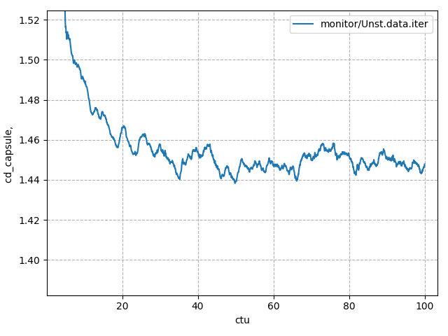
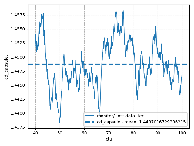
To visualize time evolution of aerodynamic loads, you can plot the time history of the drag coefficient with using the plotHist.py tool:

plotHist.py ctu cd_capsule

plotHist.py ctu cd_capsule -xRange 40 100 -showMean

References

---

1. Cheatwood, F., Winchenbach, G., Hathaway, W., and Chapman, G., "Dynamic Stability Testing of the Genesis Sample Return Capsule," 38th aerospace sciences meeting and exhibit. https://doi.org/10.2514/6.2000-1009 ↩