Gallery: Science and Engineering Powered by NASA High-End Computing
Filter media

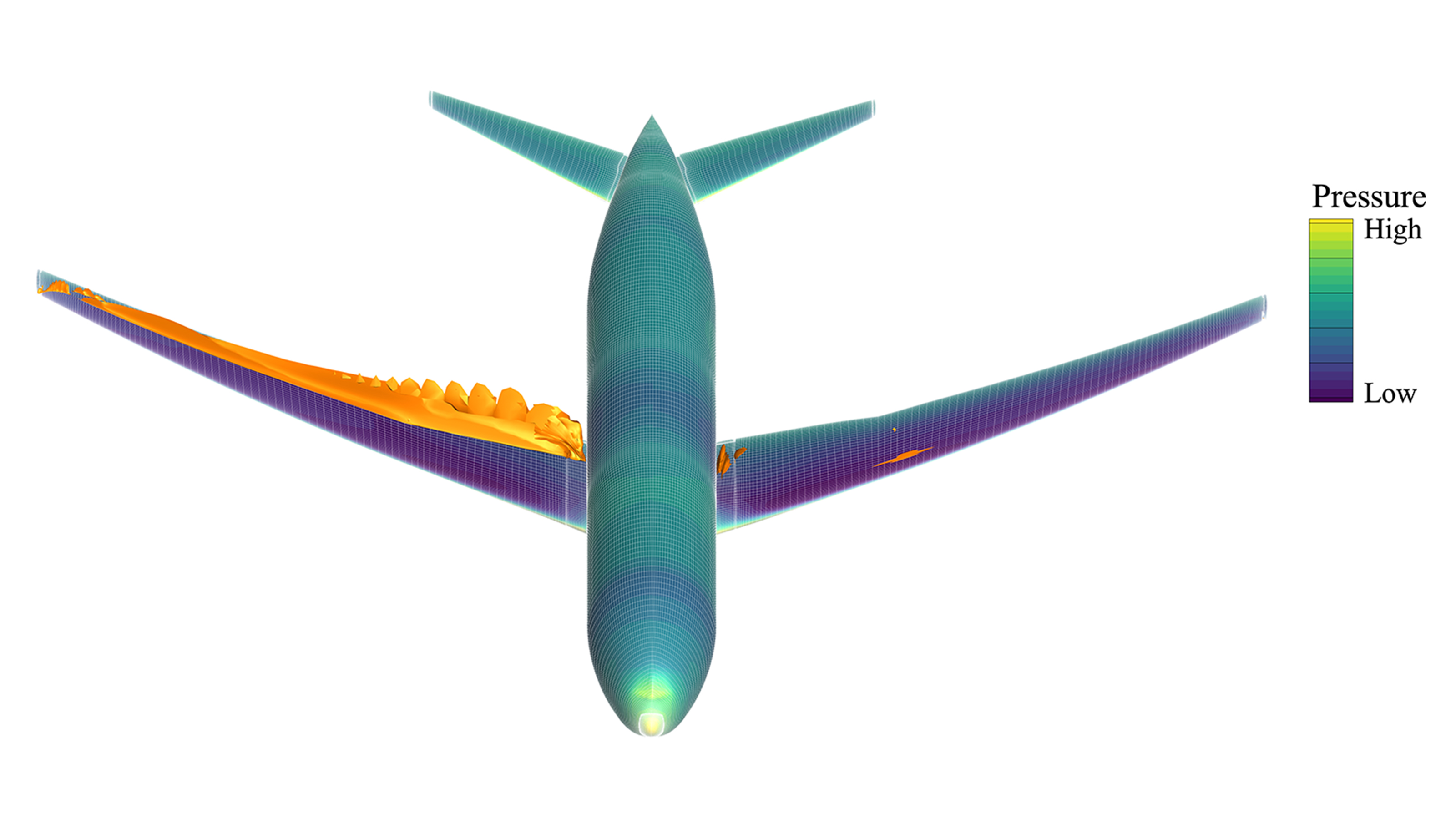
Comparison of aircraft designs colored by air pressure.
Comparison of aircraft designs: The initial geometry (left) and the optimized shape (right). The surface is colored by the air pressure on the aircraft, with orange surfaces showing shock waves. The optimized design reduces drag by 4% compared to the original, leading to improved fuel efficiency.

Read More Brandon Lowe, NASA/Ames
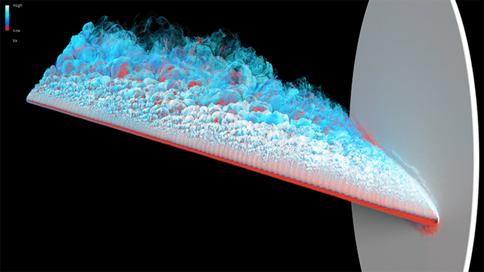
Simulation of in-flight icing on aircraft surfaces during flight.
Video of a wall-modeled large-eddy simulation of the flow over a scaled Common Research Model wing with high-fidelity leading-edge ice at an angle of attack of 8.423 degrees. This video highlights the large region of separated flow on the upper surface of the wing that forms due to the leading-edge ice. Particle tracers are injected near the leading-edge ice and advected downstream. Particles are colored by streamwise velocity, where red indicates lower velocity, and the increasingly lighter blue indicates higher velocity (with white indicating very high velocity).

Read More David Craig Penner and Timothy A. Sandstrom, NASA/Ames
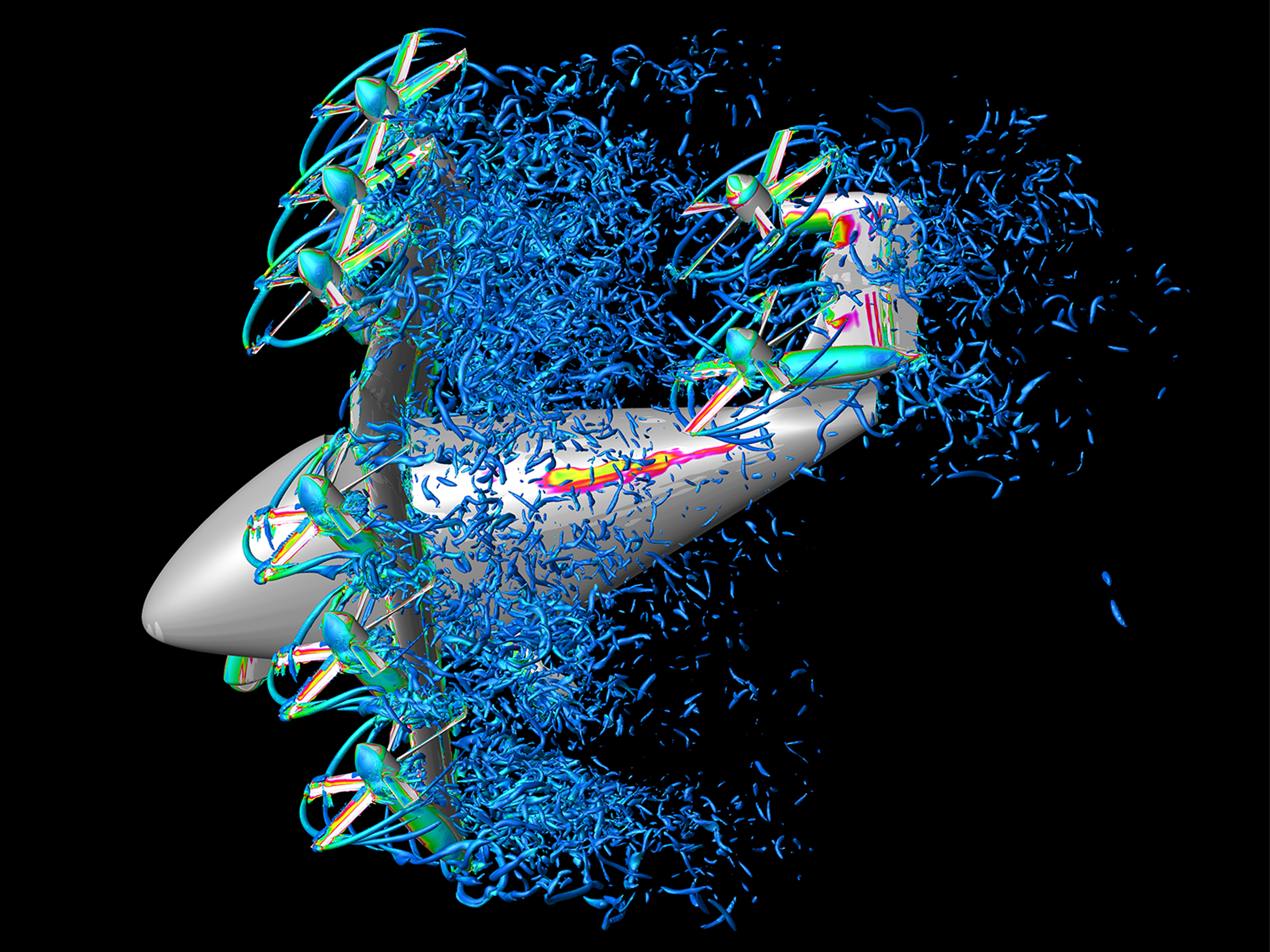
Side-oblique view of a tilt-wing urban air mobility vehicle during the transition from hover to forward flight.
Side-oblique view of a tilt-wing urban air mobility vehicle during the transition from hover to forward flight. The vortex wake is visualized by Q-criterion iso-surfaces, colored with vorticity magnitude, where blue is low and magenta is high. The simulation represents the tiltwing at an early transition stage, with the wing rotated to 60°.

Read More David Garcia Perez and Patricia Ventura Diaz, NASA/ Ames
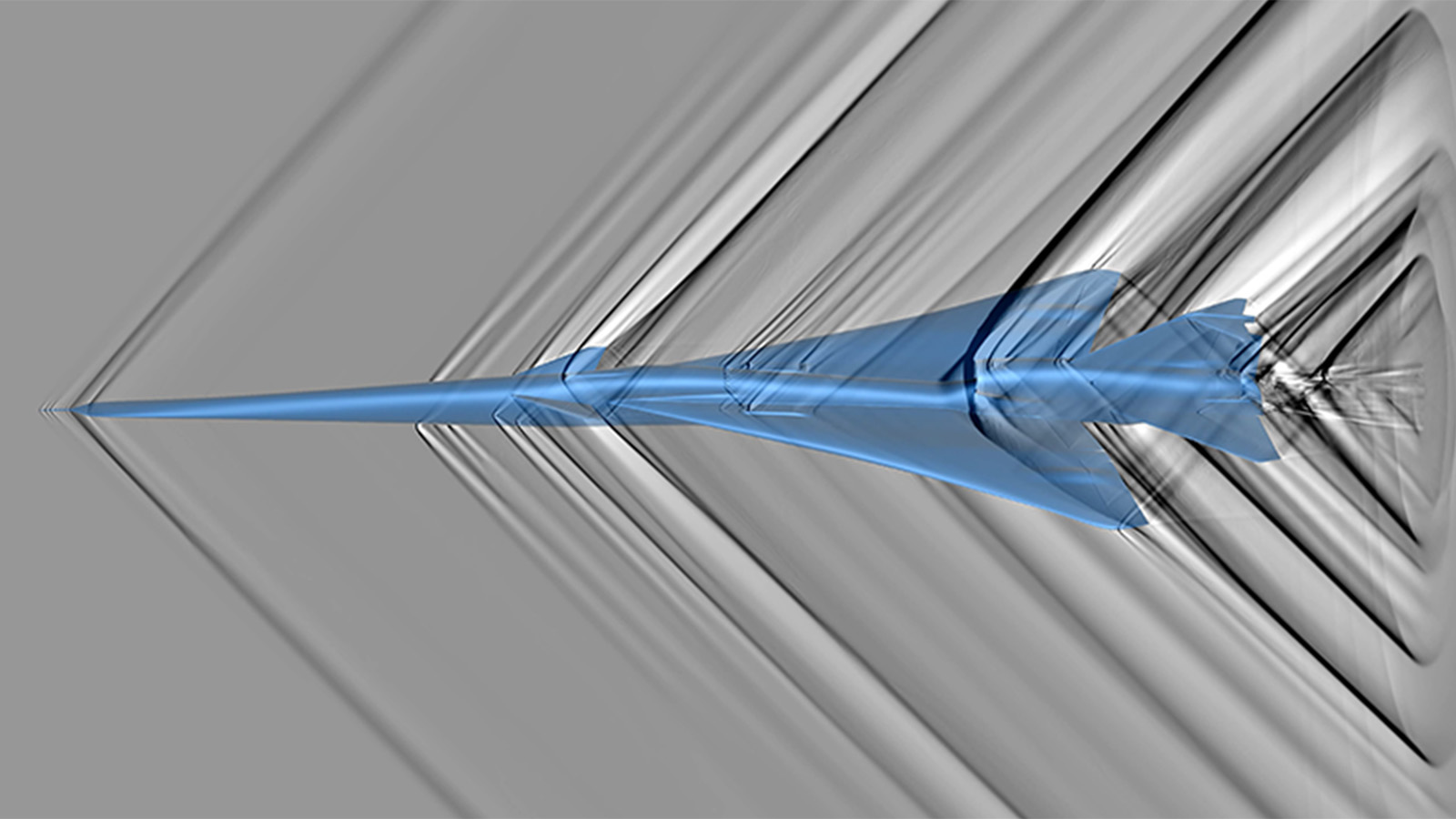
Shadowgraph simulation of a detailed computational model of the X-59 aircraft, showing shockwaves (dark lines correspond to discontinuous pressure jumps) and expansions (white regions).
Shadowgraph simulation, similar to a schlieren photograph, of a detailed computational model of the X-59 aircraft, showing shockwaves (dark lines correspond to discontinuous pressure jumps) and expansions (white regions). Note that shockwaves from the lower surface of the aircraft and much weaker than those from the upper surface, resulting in lower noise on the ground.

Read More Marian Nemec, Patrick Moran, NASA/Ames
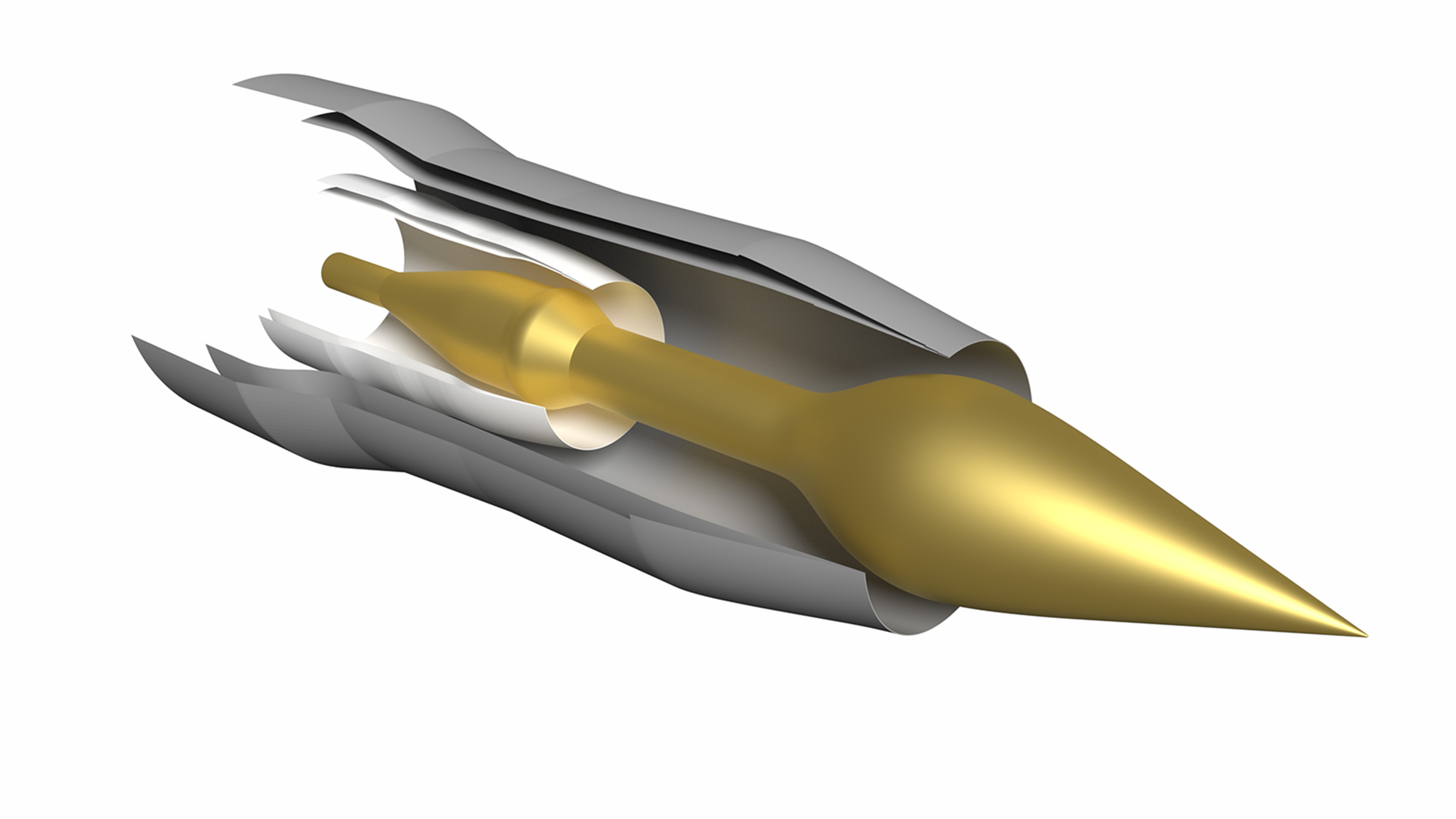
Model of the 122DLm5p2069 hot geometry jet nozzle concept with a drooped and extended plug configuration.
Model of the 122DLm5p2069 hot geometry jet nozzle concept with a drooped and extended plug configuration. Internal to the nozzle geometry is the m5 lobed mixer, which makes traditional structured overset gridding methods difficult and expensive due to the complex lobe structures.

Read More Timothy A. Sandstrom, NASA/Ames
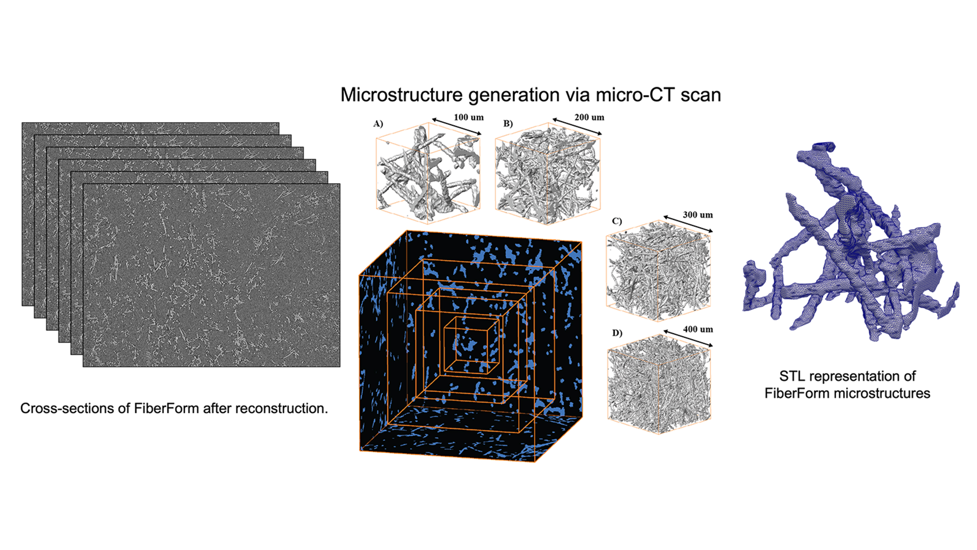
Examples of methods used to characterize the microscale architecture of thermal protection system materials and quantifying manufacturing variabilities through stochastic modeling.
Examples of methods used to characterize the microscale architecture of thermal protection system materials and quantifying manufacturing variabilities through stochastic modeling: a multitude of primary structures obtained using XRCT to obtain the primary dataset (left), extraction of volumes from the primary structure to obtain the probability distribution functions (middle), and a surface mesh generated on the extracted volumes (right).

Read More Luis Chacon and Savio Poovathingal, University of Kentucky
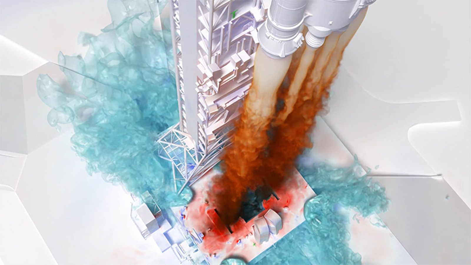
Lofted Artemis I launch simulation using the LAVA Cartesian computational fluid dynamics solver.
Lofted Artemis I launch simulation using the LAVA Cartesian computational fluid dynamics solver. The image shows a slice through the exhaust plumes where the black line indicates the 90% plume exhaust/air interface. The plume gas and launchpad surfaces are colored by pressure, where red is high and blue is low. The water mass fraction is shown using nested isocontours in teal.

Read More Chris DeGrendele, Timothy A. Sandstrom, NASA/Ames
Simulation showing the way exhaust expands around the Starship interstage as the engines increase in power.
As the upper stage Starship engines start up, their exhaust flows out of the vents in the interstage between Starship and the lower stage booster. In this animation, the exhaust is represented by colored isosurfaces. The isosurfaces change from blue to red as the Mach number increases. As the animation progresses, it shows the way the exhaust expands around the interstage grows as the engines increase in power. Due to the low pressure at the altitude where separation occurs, the exhaust spreads out far from the vehicle, completely surrounding the lower stage booster.

Read More Jason Howison, NASA/Marshall
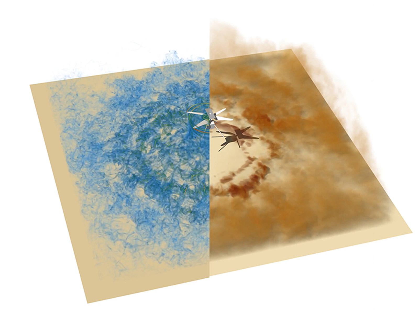
Visualization from the simulation of the Ingenuity Mars helicopter, vorticity field, and lifted dust.
Visualization from the simulation of the Ingenuity Mars helicopter hovering at a height of ℎ/𝑅 = 2, where R is the radius of the rotor, showing the vorticity field on the left (where blue is low and red is high), and lifted dust on the right (dust density is higher as the brown color intensifies), by volume rendering. The starting vortex travels downwards and interacts with the dust on the surface. The rotor wake then continues to entrain more particles from the ground, contributing to a growing cloud of dust.

Read More D. G. Caprace, Patricia Ventura Diaz, NASA/Ames
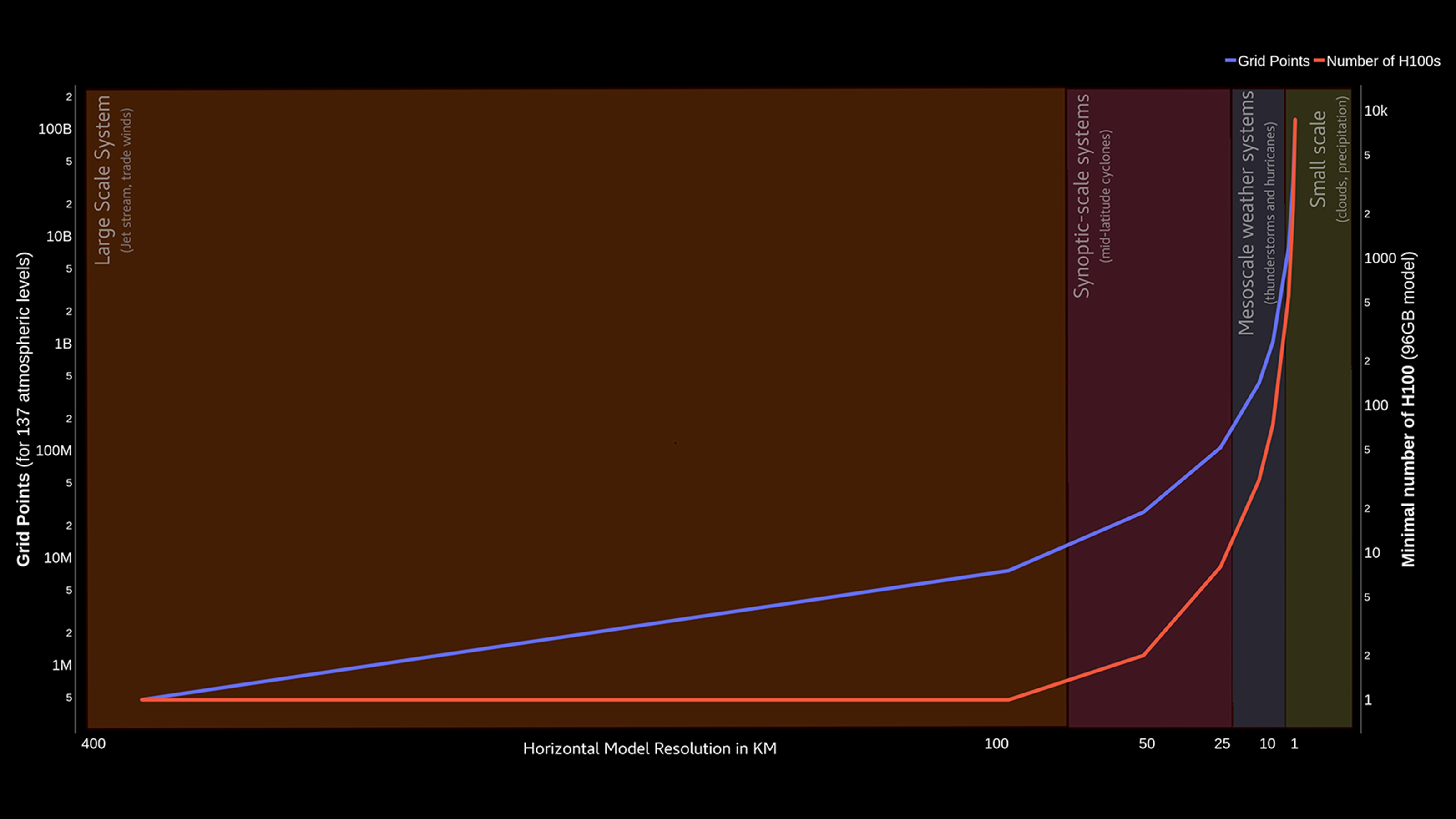
Graph comparing computational complexity vs. scientific target.
Computational complexity (expressed in both grid points to compute and minimum GPUs required) vs. scientific target (expressed in horizontal model resolution, with an overlay showing the physical processes that can be described as model resolution improves).

Read More Florian Deconinck, NASA/Goddard
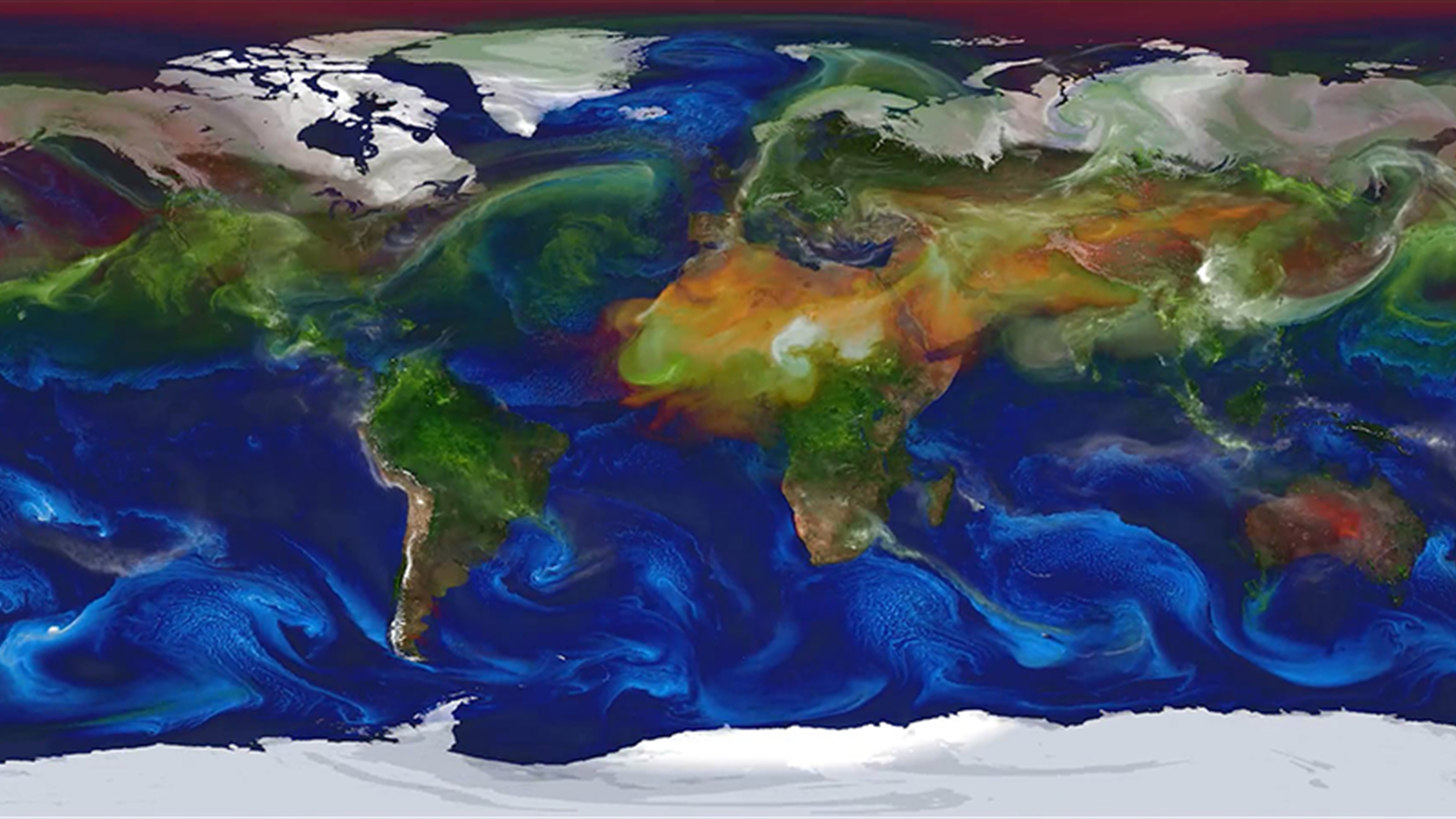
Simulation modeling global aerosols from March 1, 2007 to June 16, 2007.
This Goddard Earth Observing System (GEOS) model global aerosols simulation spans March 1, 2007–June 16, 2007. These aerosols — particles suspended in Earth’s atmosphere — can be emitted from natural sources like sea salt and pollen or from anthropogenic sources such as combustion and land use change. Aerosols influence Earth’s atmospheric composition, can absorb or reflect incoming solar radiation, and serve as the building blocks for cloud formation. NASA uses constrained simulations of aerosols as a crucial component of predicting atmospheric chemistry and physics related to climate change. Researchers are making machine learning enhancements to GEOS focused on representation of cloud formation and atmospheric composition.

Read More William Putman, NASA/Goddard
Figure illustrating true vs. predicted (non-dimensionalized) momentum fluxes in the upper troposphere (12-kilometer height).
From the Prithvi WxC foundation model’s gravity wave flux parameterization, the figure illustrates true vs. predicted (non-dimensionalized) momentum fluxes in the upper troposphere (12-kilometer height). Panels (a) and (c) show the fluxes u′ω′ and v′ω′ from the ERA5 reanalysis, and panels (b) and (d) show the respective predictions from the fine-tuned model. All fluxes are monthly averaged for May 2015. The vertical derivative of the fluxes represents the wind-forcing tendencies due to atmospheric gravity waves and can represent a portion of unresolved sub-grid tendencies in climate models.

Read More Aman Gupta, Stanford University; Sujit Roy, NASA/Marshall
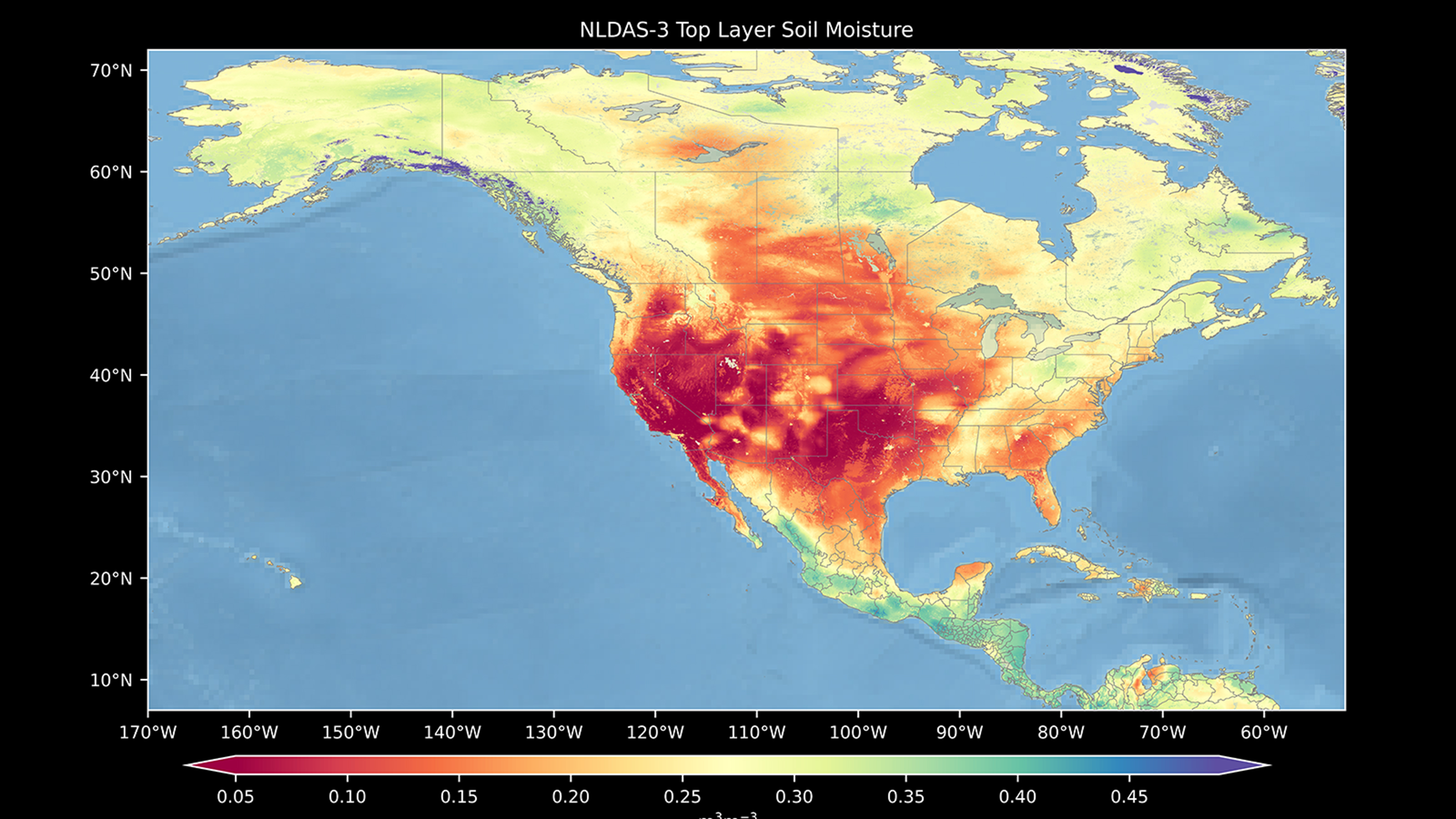
Visualization showing top-layer soil moisture from the Noah-Multiparameterization 4.0.1 land surface model.
The visualization shows top-layer (0- to 10-centimeter) soil moisture from the Noah-Multiparameterization (Noah-MP) 4.0.1 land surface model on 0z 01 Aug 1980. The red-to-blue color bar represents soil moisture. Red is dry, and blue is wet. Noah-MP is one of the models within NASA’s Land Information System framework and the North American Land Data Assimilation System.

Read More David Mocko, NASA/Goddard
A forecast of minimum lowest mean sea-level pressure (MSLP) tracing the path of Hurricane Helene.
The movie shows a NASA Goddard Earth Observing System-Forward Processing (GEOS-FP) forecast of minimum lowest mean sea-level pressure (MSLP) tracing the path of Hurricane Helene beginning nine days prior to landfall.

Read More Bill Putman, NASA/Goddard
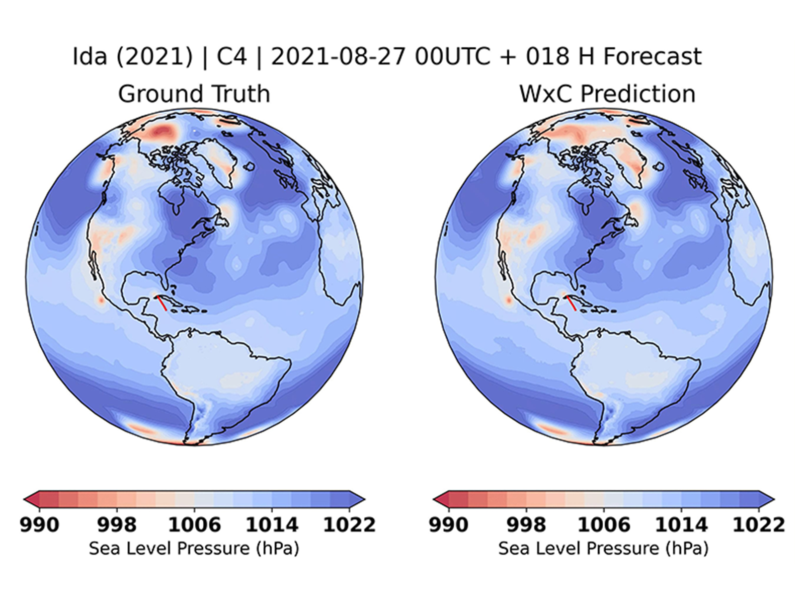
Visualization comparing the track of Hurricane Ida (2021) from MERRA-2 reanalysis data (left) with a zero-shot prediction from the Prithvi WxC foundation model (right).
This visualization compares the track of the Category 4 Hurricane Ida (2021) from MERRA-2 reanalysis data (left) with a zero-shot prediction from the Prithvi WxC foundation model (right). Both models were initialized at 00 UTC on 2021-08-27.

Read More Ankur Kumar, The University of Alabama in Huntsville; Sujit Roy NASA/Marshall
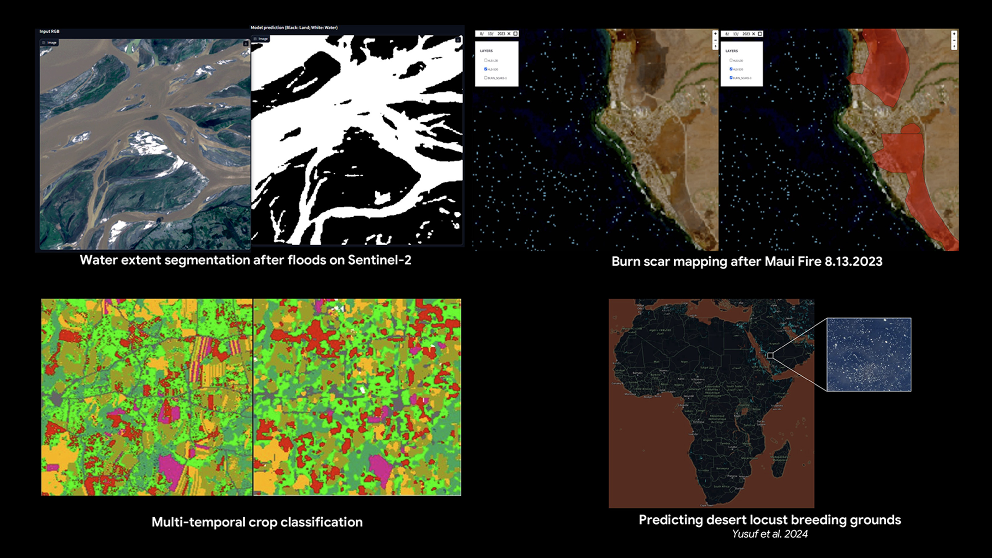
The image shows several applications of the satellite data incorporated into Prithvi. Clockwise from left to right: a) water extent segmentation after floods from Sentinel-2; b) burn scar mapping after the Maui fire on August 13, 2023; c) predicting desert locust breeding grounds (Yusuf et al. 2024); and d) multi-temporal crop classification.

Read More Paolo Fraccaro, IBM Research; Sujit Roy, NASA/Marshall
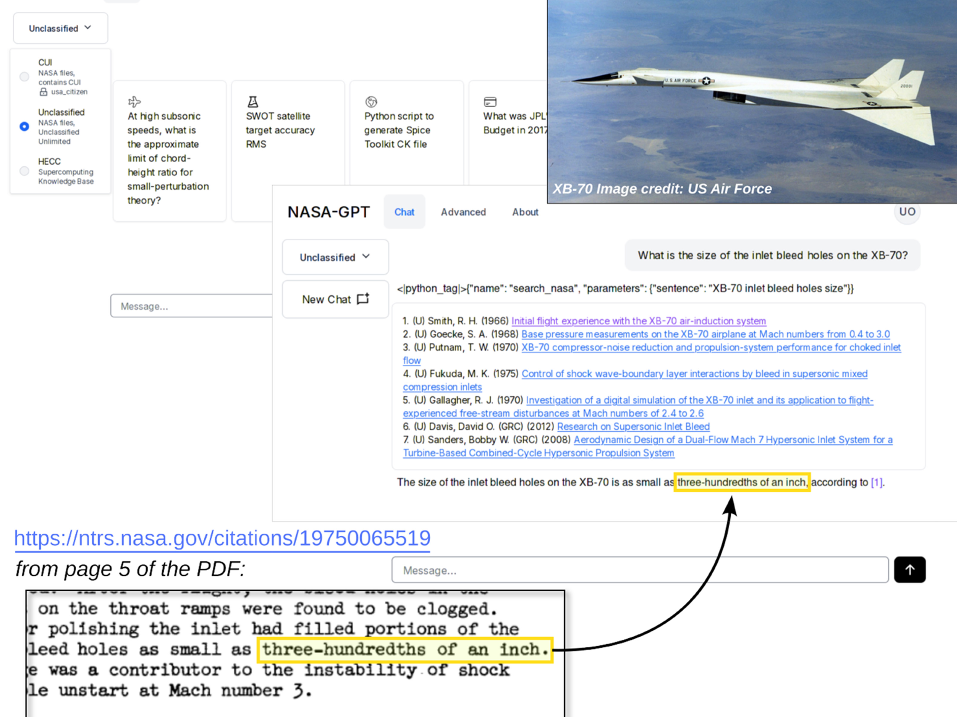
Collage representing the capabilities of NASA-GPT.
Demonstration of NASA-GPT, which has access to the entire NASA Technical Reports Server, answering a specific design question about a retired experimental aircraft from a paper written in 1966. This particular question was helpful for a current NASA civilian hypersonic aircraft project.

Read More Derek Dalle, NASA/Ames 
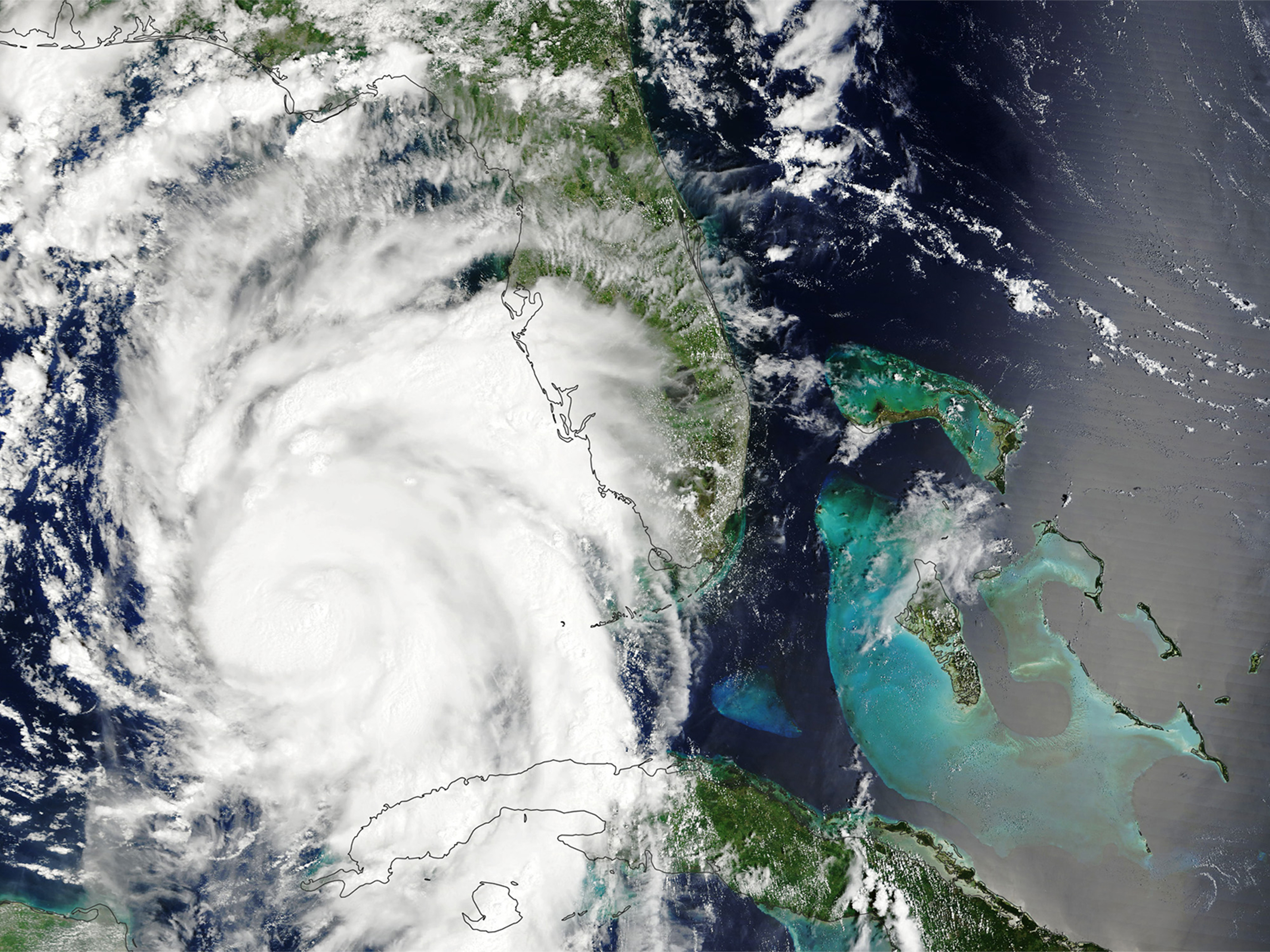
Satellite image of Hurricane Idalia in August 2023.
With the Prithvi WxC weather-climate foundational model, researchers will be able to support many climate applications that can be used throughout the science community. These applications include detecting and improving models for severe weather patterns or natural disasters such as hurricanes. NASA’s Terra satellite acquired this image of Hurricane Idalia in August 2023.

Read More NASA Earth Observatory
A global map showing concentrations of carbon dioxide as the gas moved through Earth’s atmosphere.
DYAMOND Global Carbon Dioxide: This global map shows concentrations of carbon dioxide as the gas moved through Earth’s atmosphere from January–March 2020, driven by wind patterns and atmospheric circulation. Because of the model’s high resolution, you can zoom in and see carbon dioxide emissions rising from power plants, fires, and cities, then spreading across continents and oceans. “You see here how everything is interconnected by these different weather patterns,” said NASA climate scientist Lesley Ott.

Read More NASA Scientific Visualization Studio, NASA/Goddard

Recently installed Grace Hopper racks for the Cabeus supercomputer at the NASA Advanced Supercomputing (NAS) facility at NASA Ames Research Center, Moffett Field, California.
This photo shows recently installed Grace Hopper racks for the Cabeus supercomputer at the NASA Advanced Supercomputing (NAS) facility at NASA Ames Research Center, Moffett Field, California. It will soon be joined by a similar system at the NASA Center for Climate Simulation (NCCS) at NASA Goddard Space Flight Center, Greenbelt, Maryland.

Read More Davin Chan, NASA/Ames
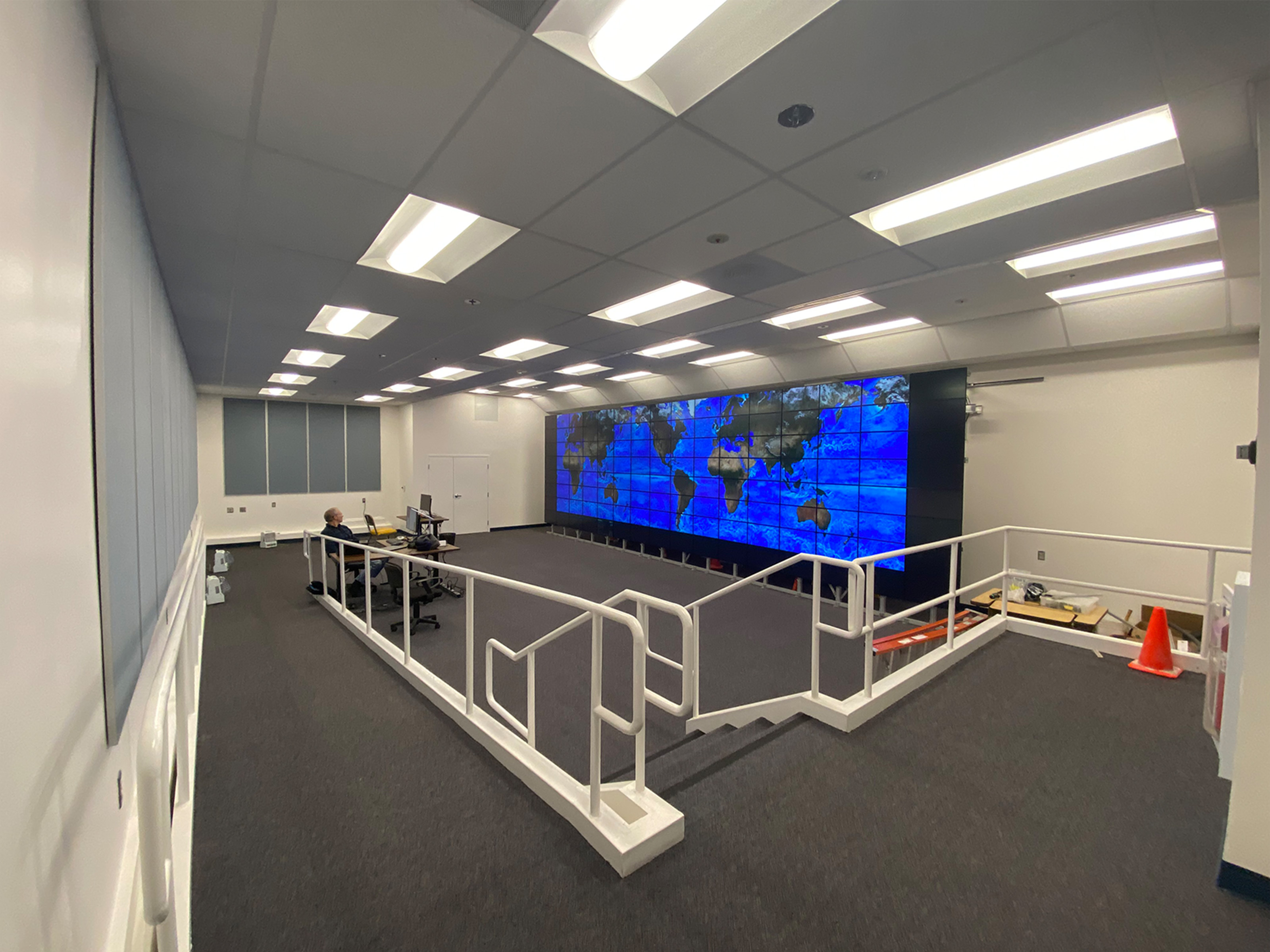
The remodeled visualization lab at the NASA Advanced Supercomputing facility, showing the new 300-square-foot hyperwall that contains over a billion pixels.
The remodeled visualization lab at the NASA Advanced Supercomputing facility, showing the new 300-square-foot hyperwall that contains over a billion pixels. The renovation involved significant changes to accommodate the new hyperwall, including removing the raised floor, increasing the floor-to-ceiling height by two feet, and installing a new ceiling.

Read More Chris Tanner, NASA/Ames
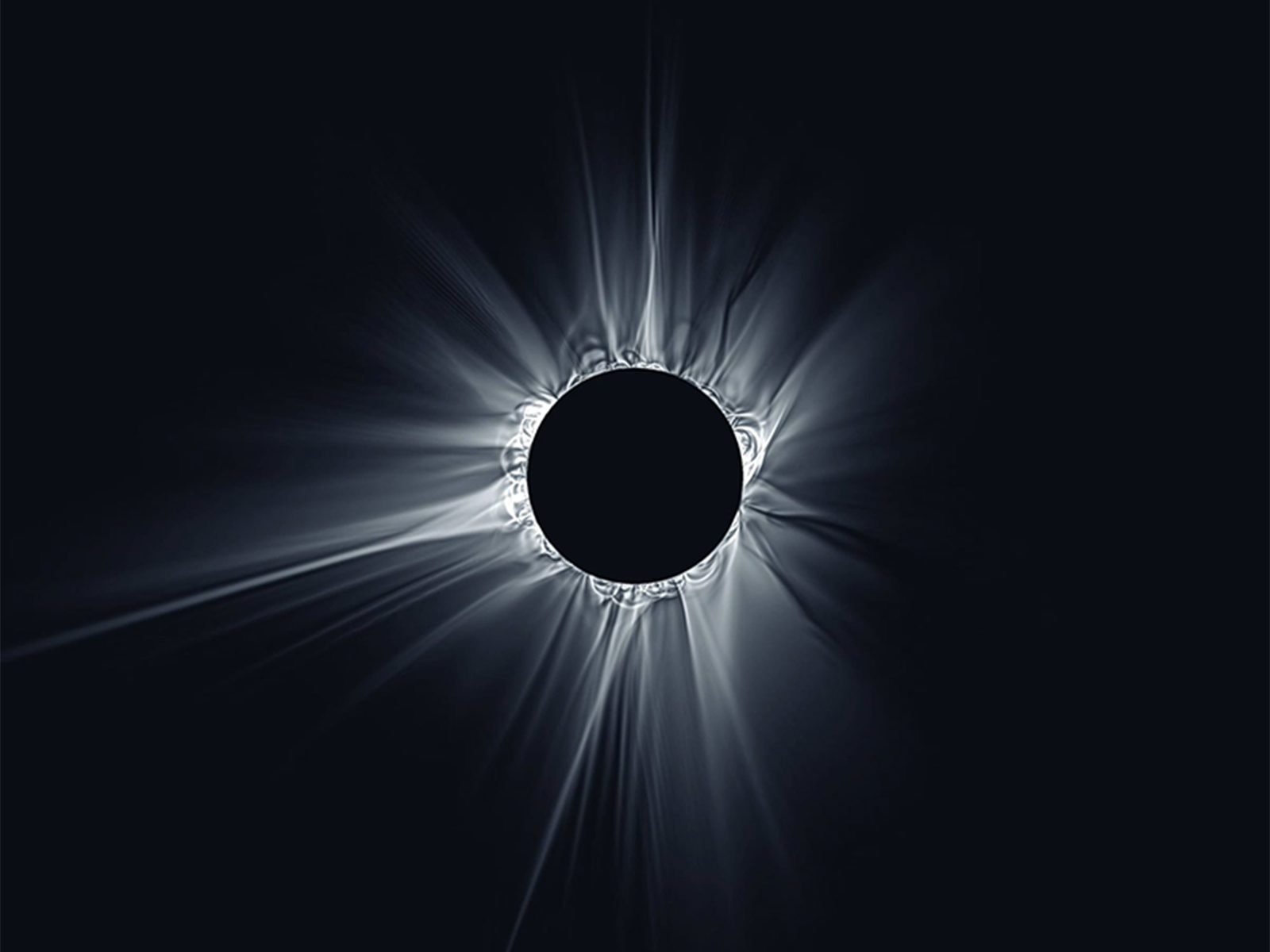
A near real-time magnetohydrodynamic (MHD) simulation predicting the appearance of the solar corona leading up to a solar eclipse.
Wavelet-processed white light emissions from the time-dependent magnetohydrodynamic model, as seen from Earth’s position on eclipse day. As the date of the eclipse gets closer and more data is assimilated into the model, the more accurate the model represents the corona during the eclipse.

Read More Predictive Science Inc.
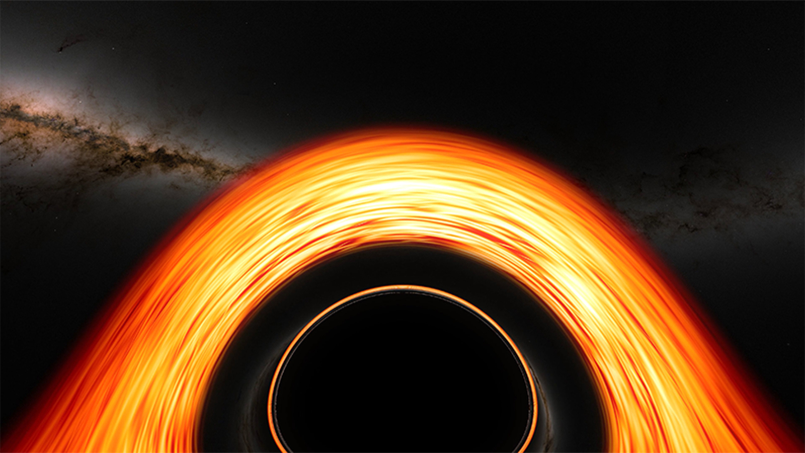
A visualization of a flight toward a supermassive black hole showing many of the fascinating features produced by the effects of general relativity.
This visualization of a flight toward a supermassive black hole shows many of the fascinating features produced by the effects of general relativity along the way. Produced on the NASA Center for Climate Simulation’s Discover supercomputer, the simulation tracks a camera as it approaches, briefly orbits, and then crosses the event horizon — the point of no return — of a monster black hole much like the one at the center of our galaxy.

Read More Jeremy Schnittman, Brian Powell, NASA/Goddard
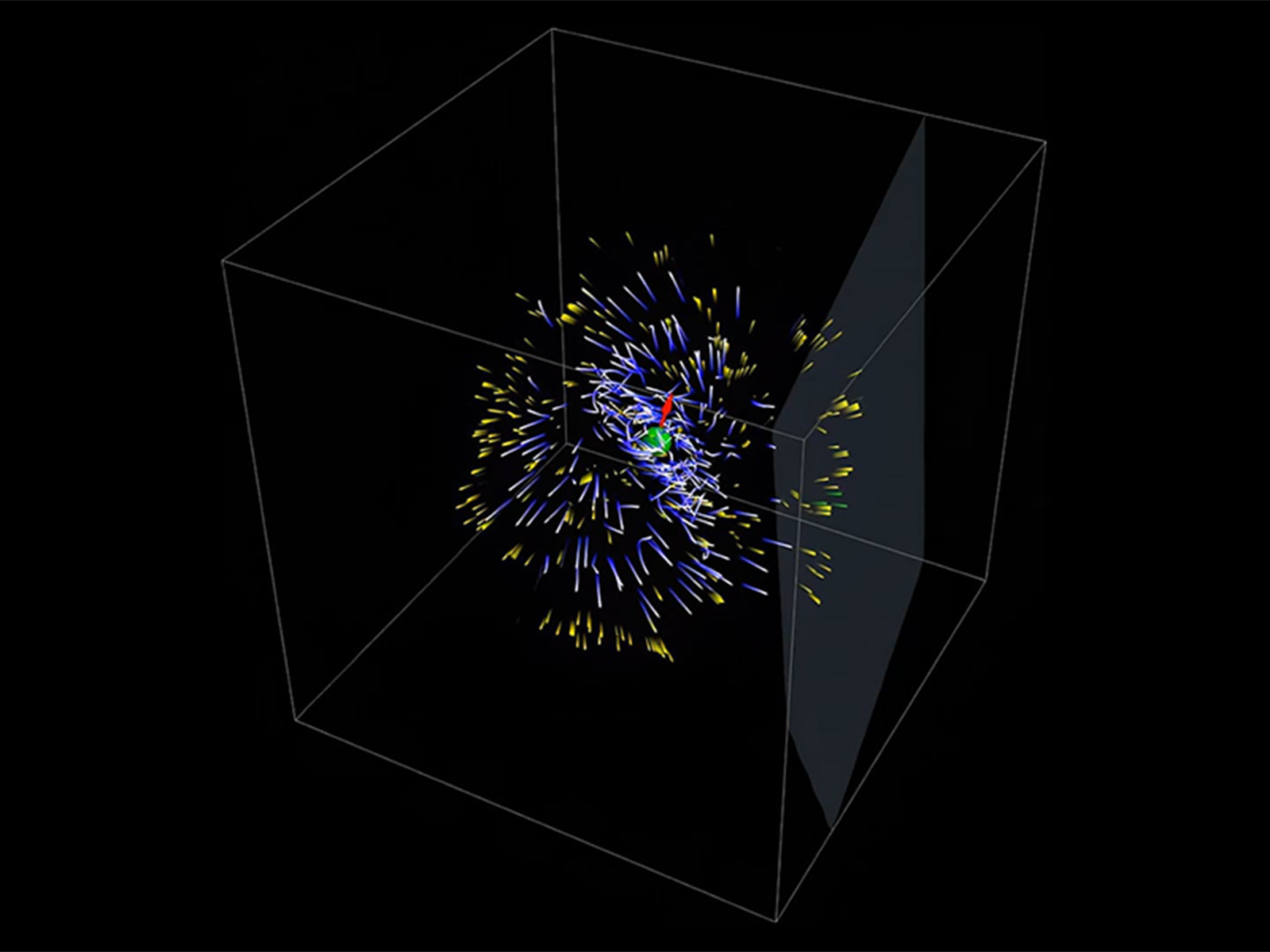
3D relativistic particle-in-cell simulations of pulsar magnetospheres over eight rotations.
This video showcases 3D relativistic particle-in-cell simulations of pulsar magnetospheres over eight rotations. The red arrow shows the direction of the star's dipolar magnetic field. Blue trajectories trace high-energy electron/positron orbits, producing gamma rays (yellow), while green rays represent photons hitting the observer's plane, illustrating how Fermi detects pulsar gamma rays.

Read More Constantinos Kalapotharakos, NASA/Goddard
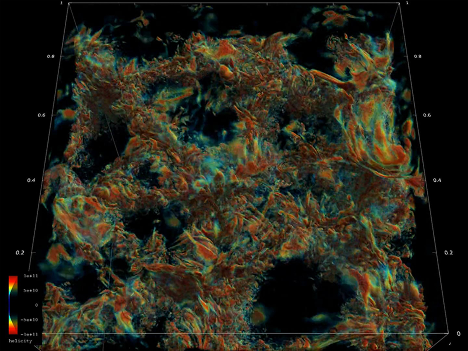
Simulation showing the evolution and coupling of the helical flows in the upper layers of the Sun’s convection zone and low atmosphere.
3D radiative hydrodynamic simulation showing the evolution and coupling of the helical flows in the upper layers of the Sun’s convection zone and low atmosphere. The sharp change of the turbulence structure in the horizontal plane corresponds to the solar surface. These turbulent flows can generate magnetic fields and excite sound waves, shock waves in the atmosphere, and eruptions. Brighter colors represent the most vigorous helical plasma motions.

Read More Irina Kitiashvili and Timothy A. Sandstrom, NASA/Ames
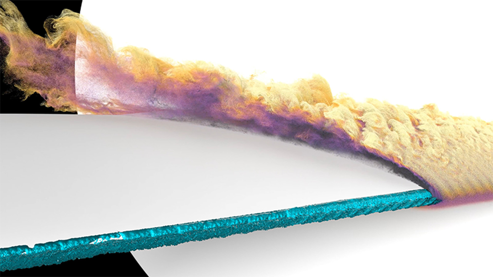
Simulation of in-flight icing on aircraft surfaces during flight.
Video of a wall-modeled large-eddy simulation of the flow over a scaled Common Research Model wing with high-fidelity leading-edge ice at an angle of attack of 8.423 degrees. This video highlights the region of separated flow that occurs immediately downstream of the leading-edge ice. Particle tracers are injected near the leading-edge ice and advected downstream. Particles are colored by streamwise velocity, where the darker color indicates lower velocity, and the lighter color indicates higher velocity.

Read More David Craig Penner and Timothy A. Sandstrom, NASA/Ames
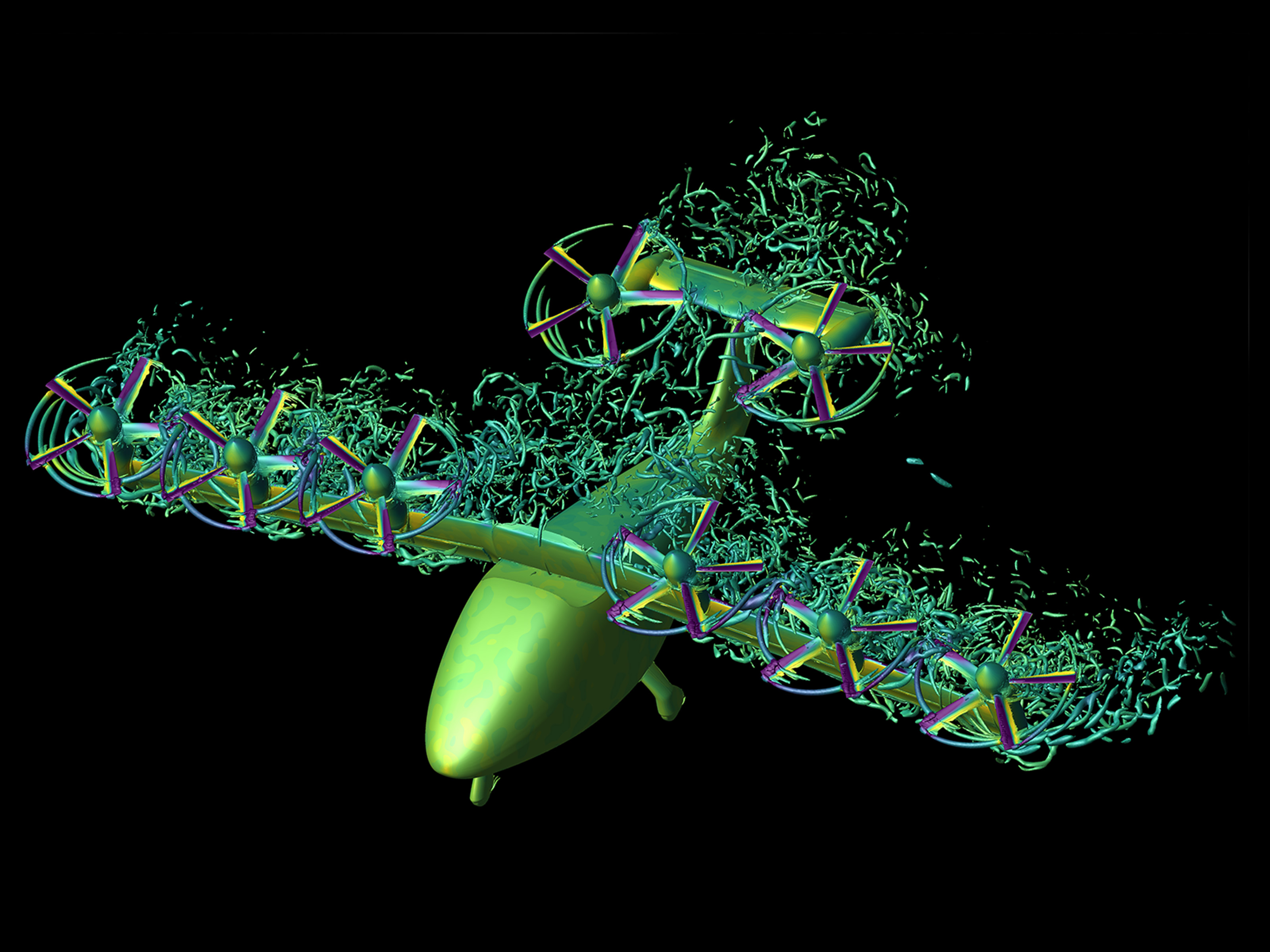
Simulation of NASA’s tilt-wing urban air mobility vehicle in transition from hover to forward flight.
Simulation of NASA’s tilt-wing urban air mobility vehicle in transition from hover to forward flight. The flow visualization shows the Q-criterion iso-surfaces colored with pressure coefficient, where purple is low and yellow is high. The pressure coefficient is also shown .

Read More David Garcia Perez and Patricia Ventura Diaz, NASA/Ames
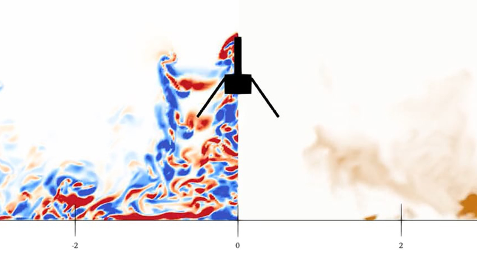
Flow visualization of the Ingenuity Mars helicopter.
Flow visualization of the Ingenuity Mars helicopter hovering at a height of ℎ/𝑅 = 2, where R is the radius of the rotor. The vertical slice shows the plane-normal vorticity on the left, and the dust density on the right. When a rotorcraft hovers above a flat surface, the flow induced by the rotor(s) is redirected from downwash in the region right underneath the rotors to outwash along the surface. In the region directly above the surface, a so-called wall jet forms with a velocity mainly pointing along the outward radial direction.

Read More D. G. Caprace, Patricia Ventura Diaz, NASA/Ames
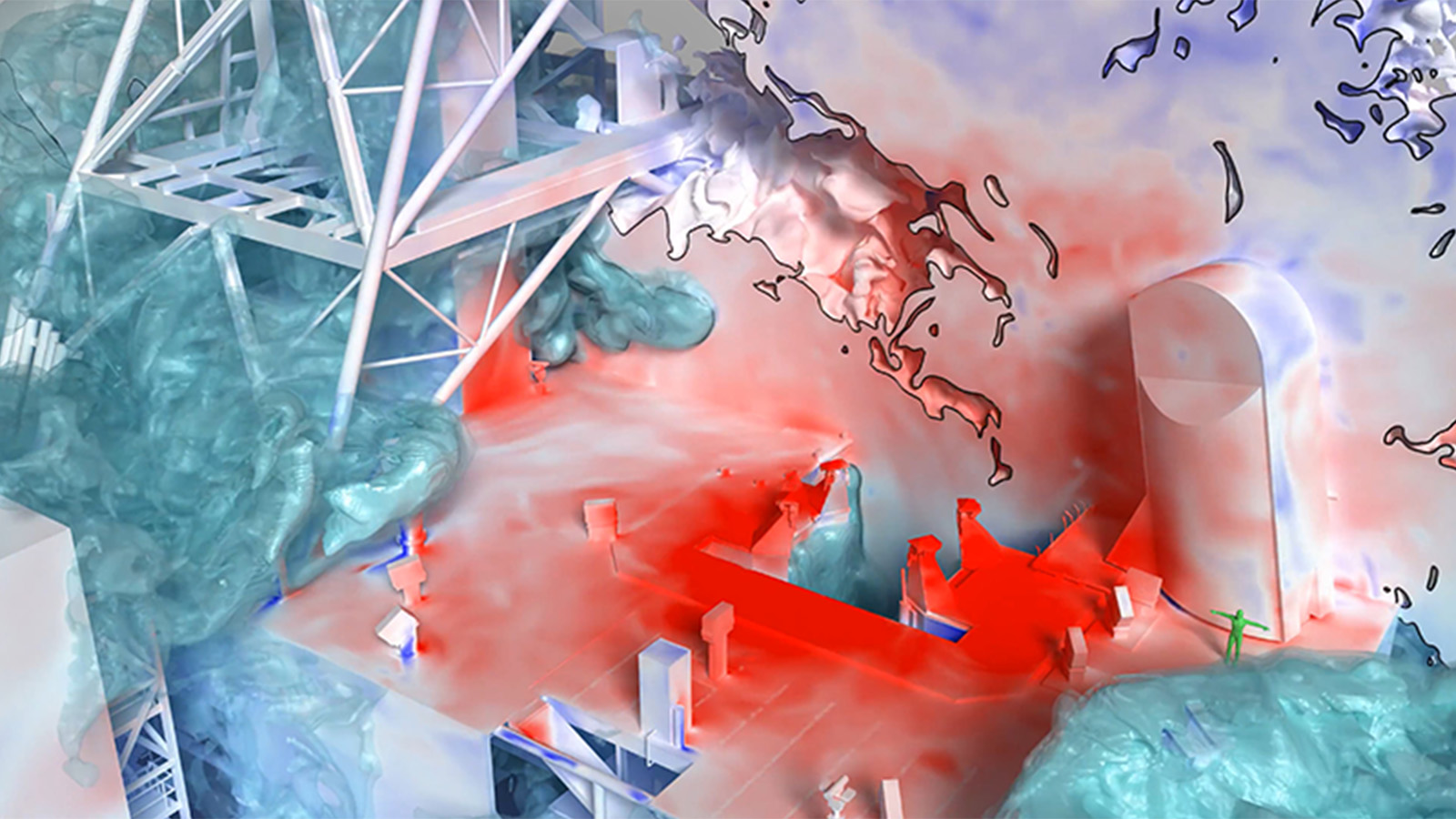
Lofted Artemis I launch simulation using the LAVA Cartesian computational fluid dynamics solver.
Lofted Artemis I launch simulation using the LAVA Cartesian computational fluid dynamics solver. The image shows a slice through the exhaust plumes where the black line indicates the 90% plume exhaust/air interface. The plume gas and launchpad surfaces are colored by pressure, where red is high and blue is low. The water mass fraction is shown using nested isocontours in teal.

Read More Chris DeGrendele, Timothy A. Sandstrom, NASA/Ames
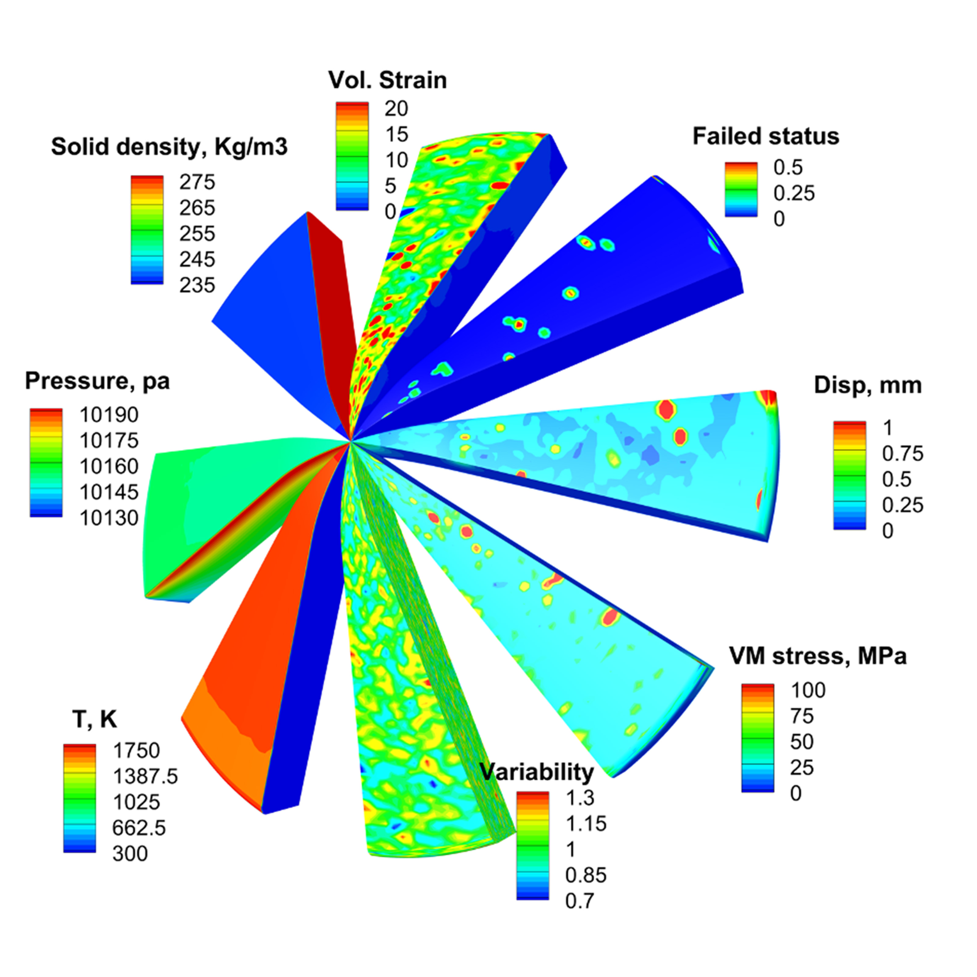
An example of stochastic modeling for a thermal protection system using a multi-scale approach to quantify material reliability.
An example of stochastic modeling for a thermal protection system using a multi-scale approach to quantify material reliability, with each slice showing the thermal-mechanical-chemical behavior within the material during a single simulation.

Read More Rick Fu and Alexandre Martin, University of Kentucky
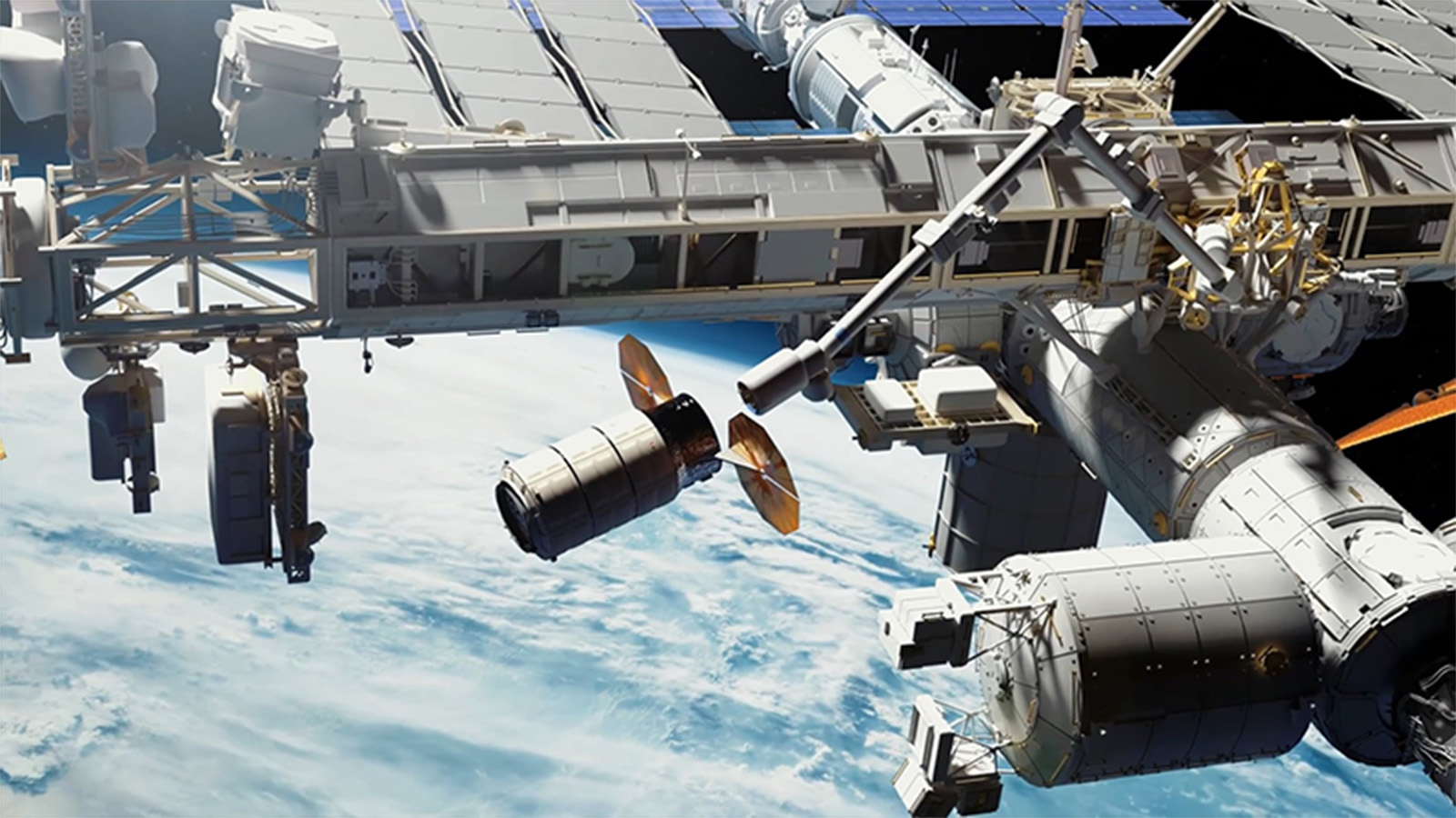
This video depicts the Concept of Operations (CONOPS) of the Kentucky Re-entry Universal Payload System.
This video depicts the Concept of Operations (CONOPS) of the Kentucky Re-entry Universal Payload System, the re-entry hypersonic vehicle developed at the University of Kentucky—from blast off to splashdown back on Earth.

Read More Alexandre Martin and Savio Poovathingal, University of Kentucky
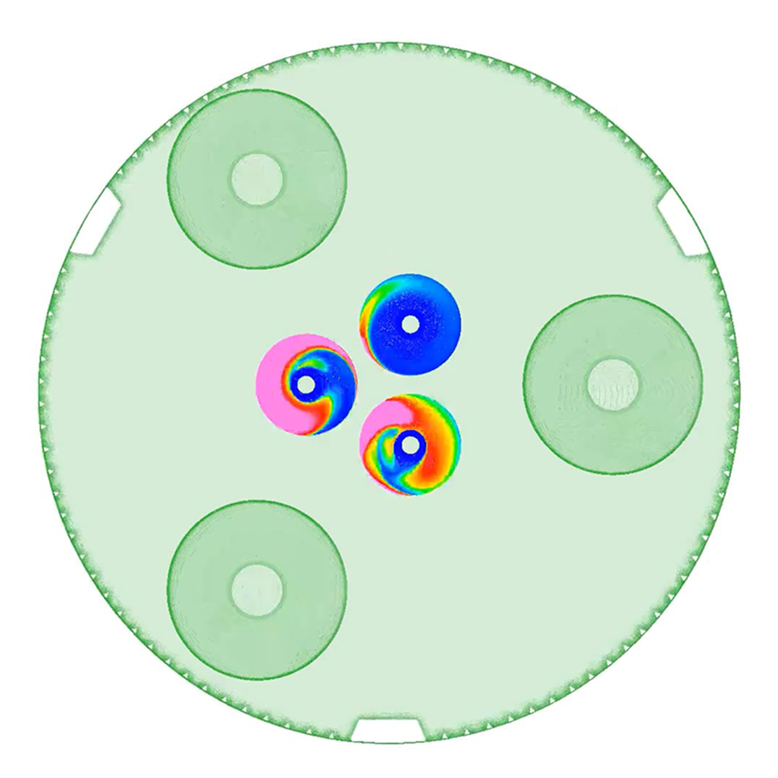
In this animation, red indicates where hot gas from the outer engines impinges on the inner engine nozzle walls.
As the engines start up, the flow inside the interstage becomes quite complex. Flow from the outer vacuum engines interacts with the walls of the non-firing inner engines. In this animation, red indicates where hot gas from the outer engines impinges on the inner engine nozzle walls. As the engines start up, swirling flow develops inside the nozzles of the inner sea-level engines.

Read More Jason Howison, NASA/Marshall
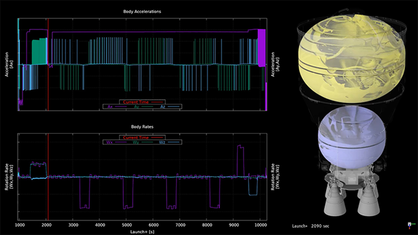
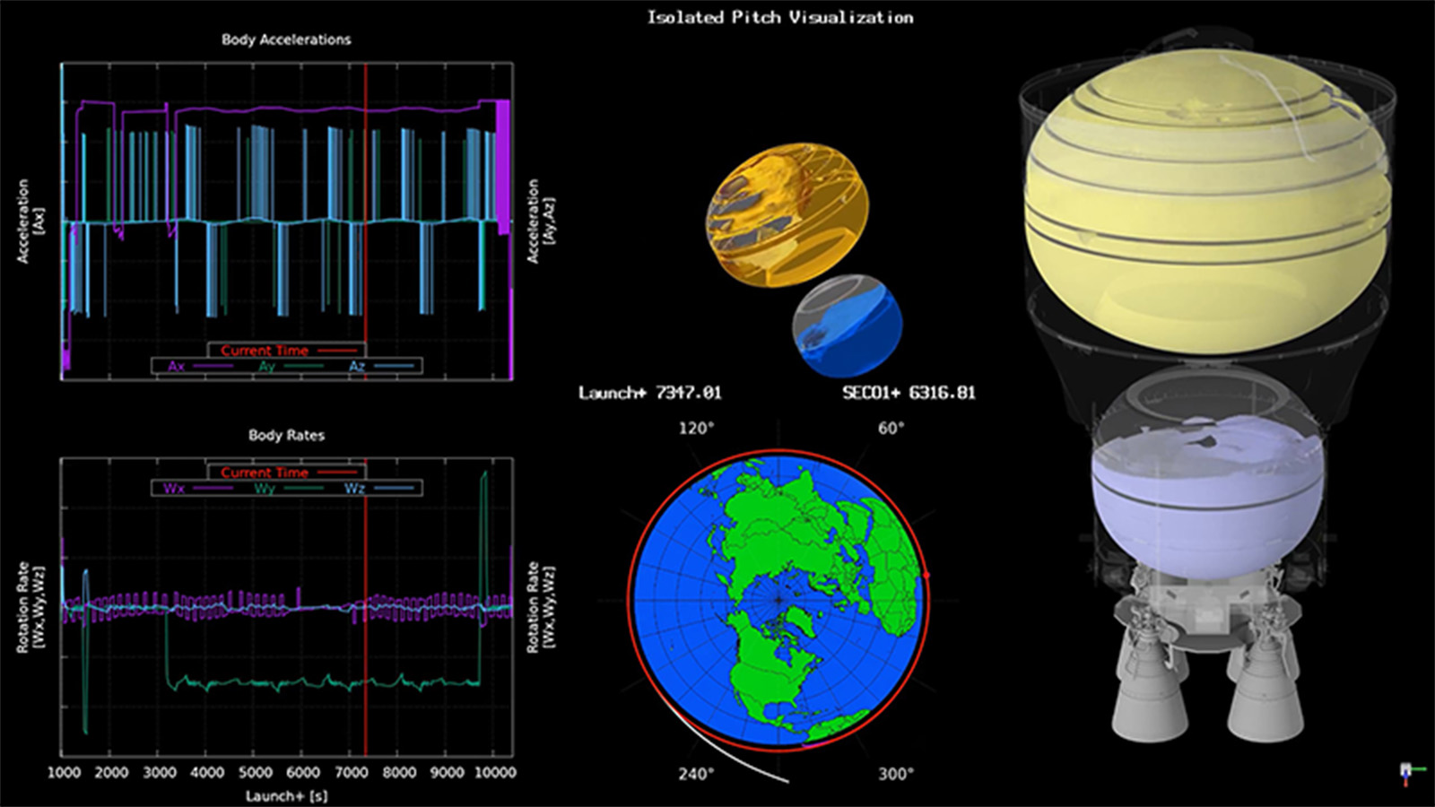
“Fishbowl” style animation of the two Space Launch System Exploration Upper Stage propellant tanks.
“Fishbowl” style animation of the two Space Launch System Exploration Upper Stage propellant tanks (1 of 3). The simulations depict where the fluid interface is located, and on what side the liquid resides, using a combination of isosurface and wall thresholding to allow for better understanding of the fluid motion in low gravity. Next to the fluid visualizations are plots of the vehicle accelerations and body rates input to the CFD simulation. The axial acceleration profile (Ax) is depicted in the trajectory plots in purple in the top plot, with settling maneuvers pointing negative for this coordinate system. The current time is depicted by a vertical red bar.

Read More Marco Sansone, NASA/Marshall
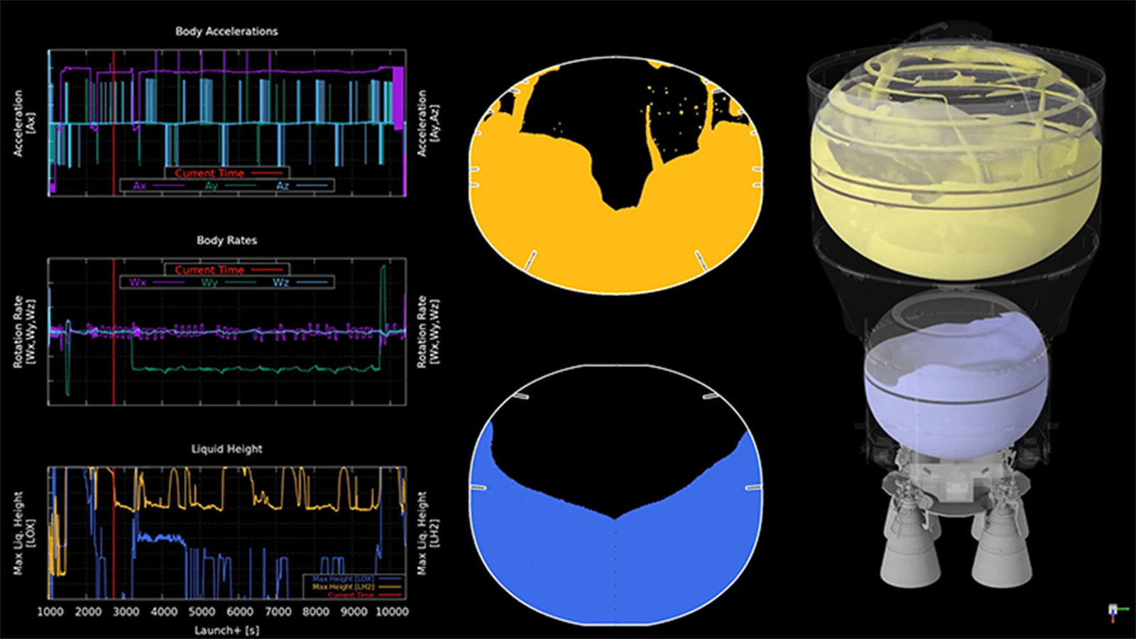
“Fishbowl” style animation of the two Space Launch System Exploration Upper Stage propellant tanks.
“Fishbowl” style animation of the two Space Launch System Exploration Upper Stage propellant tanks (2 of 3). For the same mission coast period as in (1), the analyzed trajectory inputs chosen as estimated bounding scenarios were varied for different vehicle configurations and Monte Carlo seeds. This trajectory differs from the previously shown case by a secondary Reaction Control System settling event, and a long duration pitch maneuver. The sustained pitch drives the propellant in both tanks forward, reorienting the general surface direction with the resulting centripetal force. This propellant positioning becomes unstable as the fluid is still able to climb against this force, particularly by adhering to the baffles.

Read More Marco Sansone, NASA/Marshall
“Fishbowl” style animation of the two Space Launch System Exploration Upper Stage propellant tanks.
“Fishbowl” style animation of the two Space Launch System Exploration Upper Stage propellant tanks (3 of 3). The same vehicle trajectory configuration as in (2), with an alternate Monte Carlo seed, will have minor differences in Reaction Control System thruster firing times without changing large, prescribed maneuvers, such as the long pitch described for the previous case. To better analyze the effects of this pitch maneuver, an alternate liquid position visualization method is used to clearly show axial propellant location and forward dome wetting. Rather than a simple cut plane, all circumferential points were flattened, so that if propellant exists at a given radius and axial location it is represented in the new 2D plot. The potential for propellant to cover a vent port during planned venting, like during the sustained pitching shown here, was noted from the analysis results. Methods to modify trajectories to preclude propellant venting were developed using resulting visualizations.

Read More Marco Sansone, NASA/Marshall
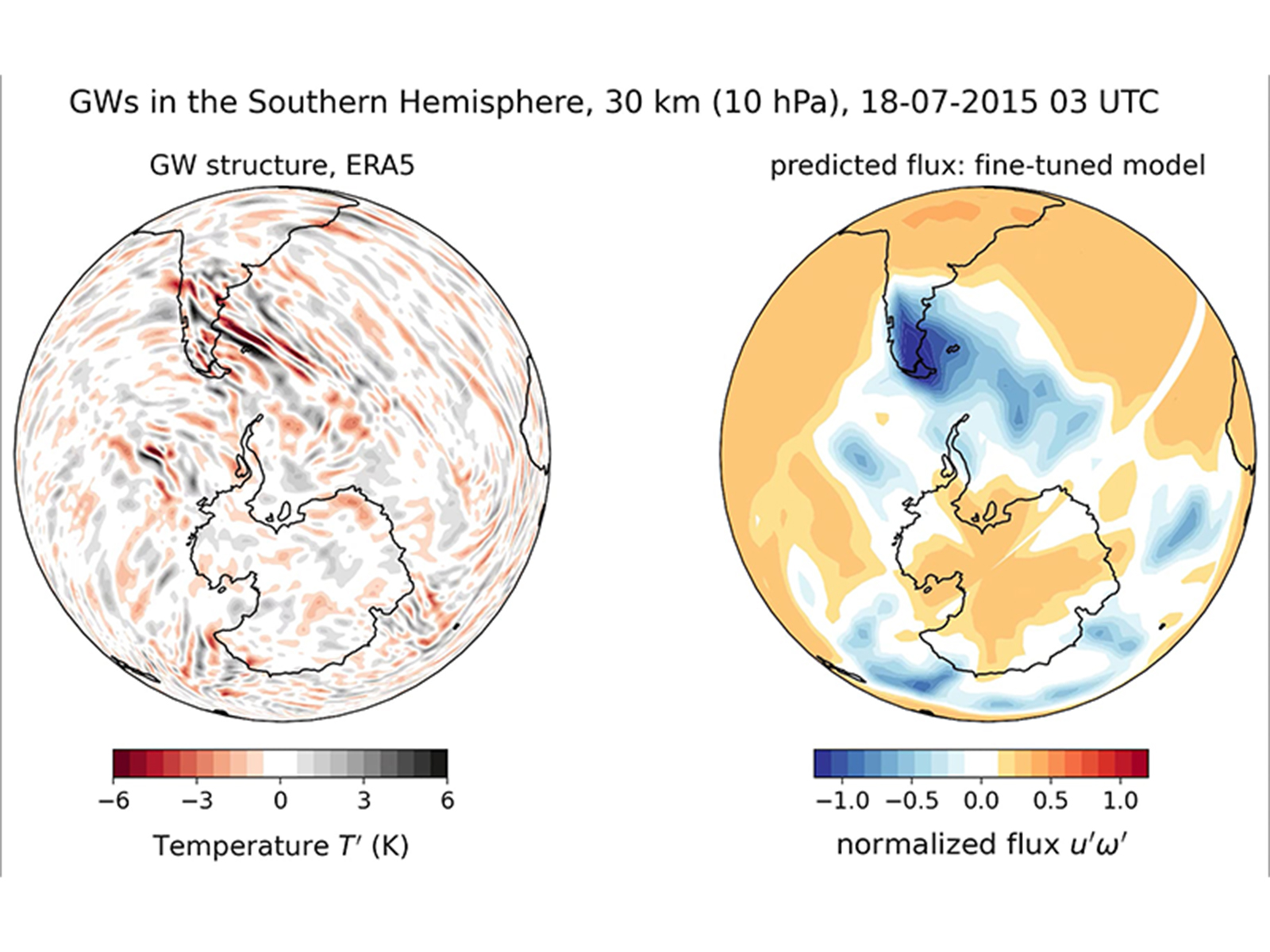
This visualization compares the baseline and fine-tuned versions of the Prithvi WxC foundation model.
This visualization compares the baseline and fine-tuned versions of the Prithvi WxC foundation model. The left plot shows gravity waves over the Andes, parts of Antarctica, and the Southern Ocean. The right plot shows predicted momentum flux (u'w') carried by these waves. The vertical derivative of the flux equates to the net wind acceleration/deceleration applied by the waves.

Read More Aman Gupta, Stanford University; Sujit Roy, NASA/Marshall
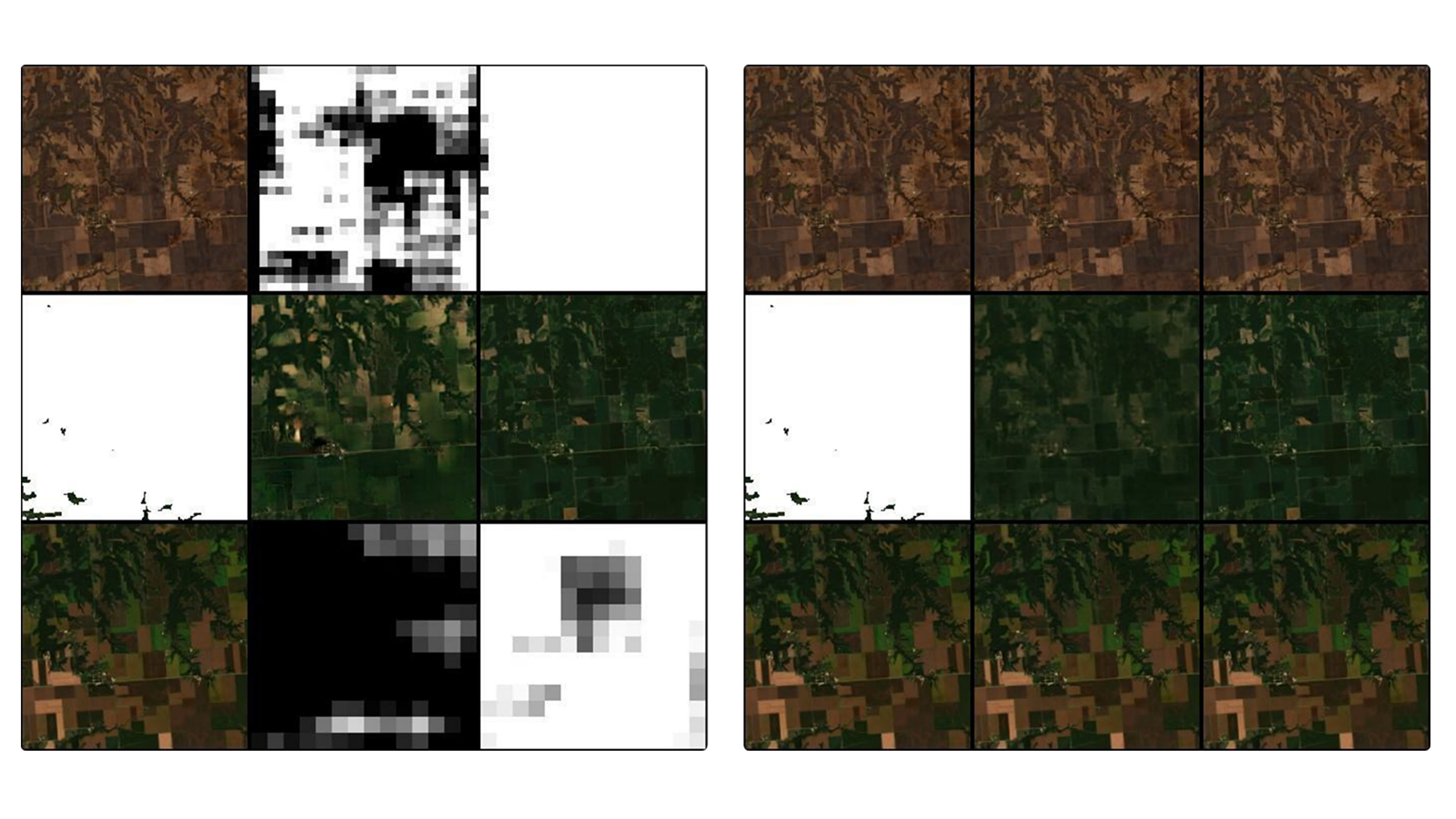
Comparison of true color composites of model outputs for Prithvi and Conditional Generative Adversarial Training (CGAN) for multi-temporal cloud gap filling.
Comparison of true color composites of model outputs for Prithvi and Conditional Generative Adversarial Training (CGAN) for multi-temporal cloud gap filling. From left to right, each three-square block shows model input, reconstruction using model output, and ground truth. Each row represents a time step.

Read More Denys Godwin, Hamed Alemohammad, Clark University
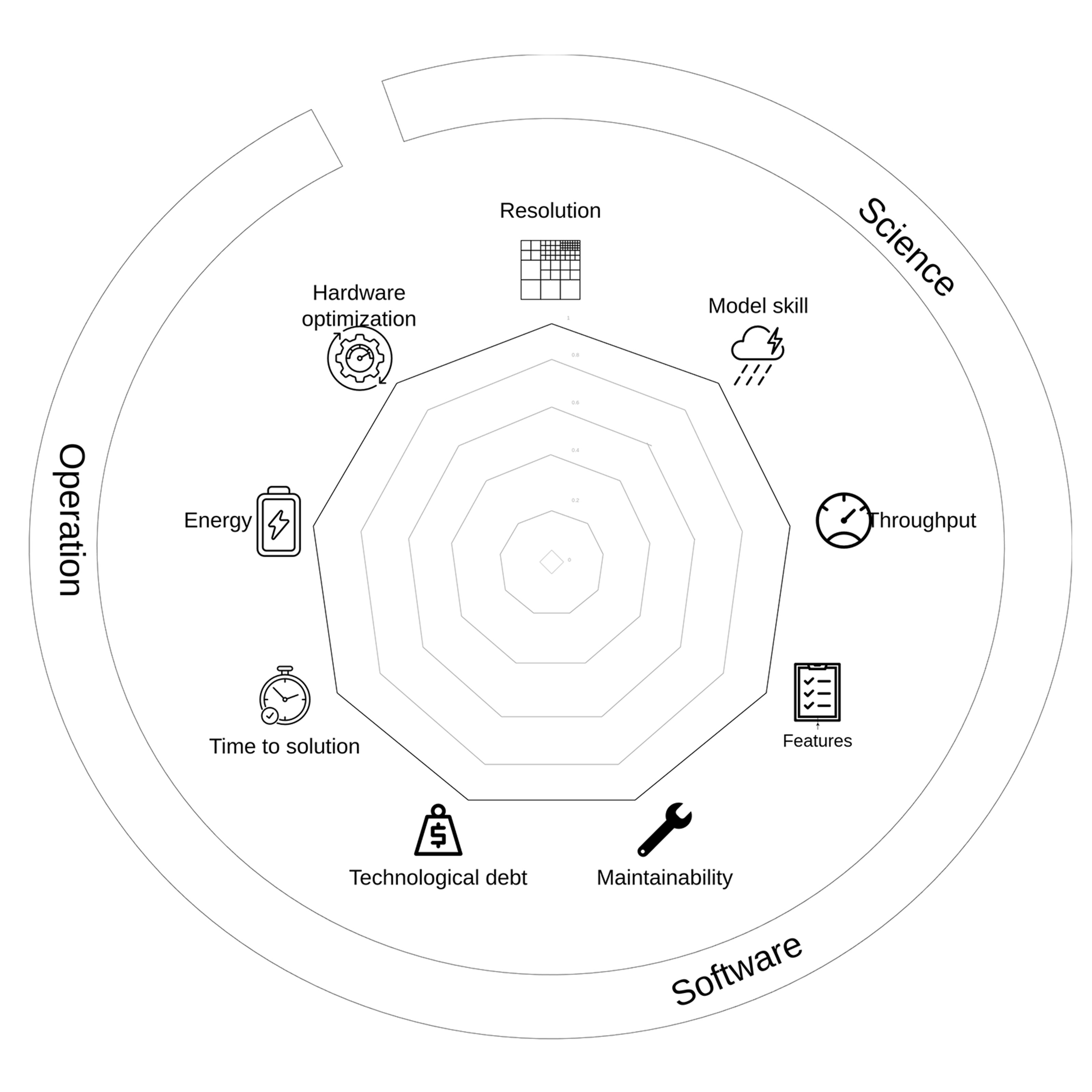
Spider graph showing the impact metrics to evaluate a project-technology coupling.
Spider graph showing the impact metrics to evaluate a project-technology coupling in three main categories: scientific target (Science), software quality (Software), and operational goals (Operation).

Read More Florian Deconinck, NASA/Goddard
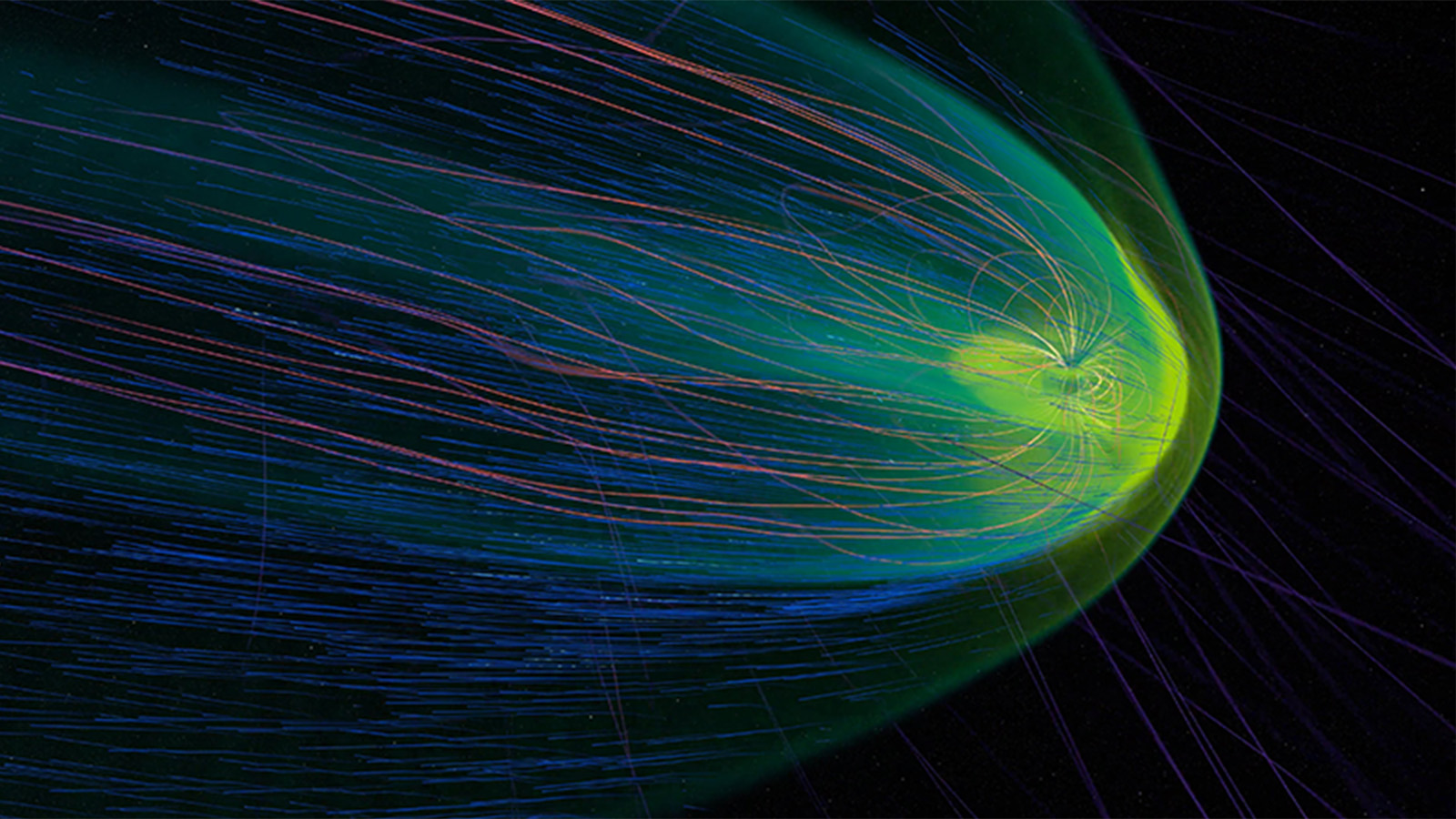
Geomagnetic Storm Causes Satellite Loss: In February 2022, a coronal mass ejection led to 38 commercial satellites being lost.
Geomagnetic Storm Causes Satellite Loss: In February 2022, a coronal mass ejection led to 38 commercial satellites being lost. Solar plasma heated the atmosphere, causing denser gases to expand into the satellites’ orbit, which in turn increased atmospheric drag on the satellites to the point of de-orbit. This data comes from the space weather-predicting Multiscale Atmosphere-Geospace Environment (MAGE) supercomputer model built by the Applied Physics Laboratory’s Center for Geospace Storms.

Read More NASA Scientific Visualization Studio, NASA/Goddard

Forward-modeled white light emission of the time-dependent magnetohydrodynamic model.
Forward-modeled white light emission of the time-dependent magnetohydrodynamic model shown from a viewpoint that NASA’s Parker Solar Probe would see at its point of orbit around the Sun closest to the date/time of the April 8, 2024 total solar eclipse.

Read More Predictive Science Inc.
This sequence shows a zoom into the camera’s direction of travel as it loops around the black hole.
This sequence shows a zoom into the camera’s direction of travel as it loops around the black hole to reveal the detailed structure of the photon rings. Each band is a distorted image of the gas disk layered between the background sky. Successive bands are thinner, produced by photons that have taken an additional trip around the black hole before reaching the camera. The field of view is 10 degrees across, about the width of a fist held at arm’s length.

Read More Jeremy Schnittman, Brian Powell, NASA/Goddard
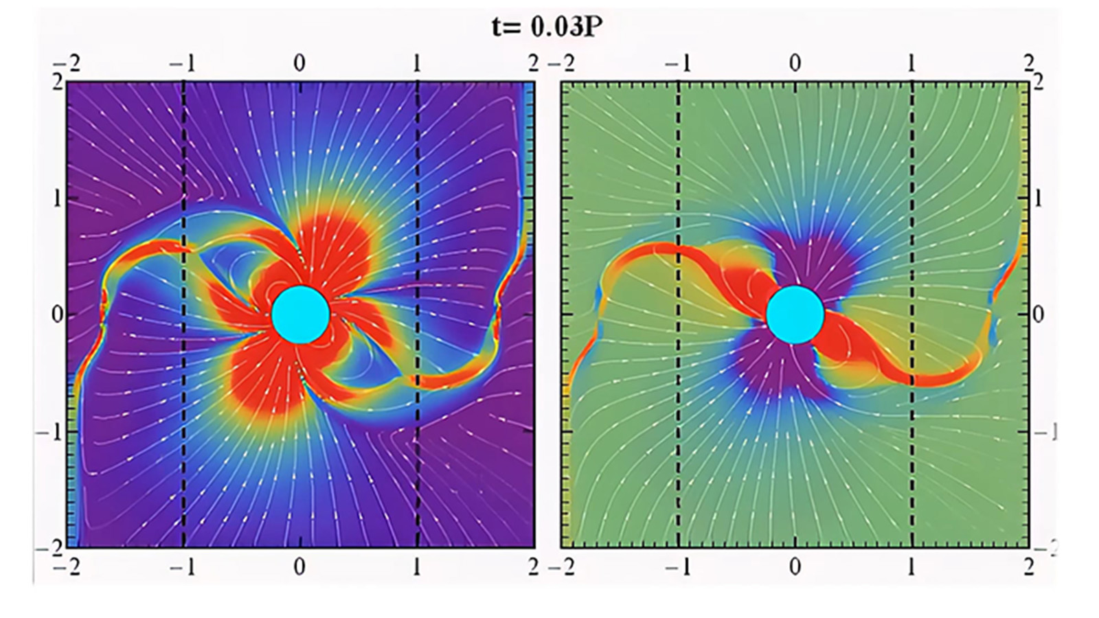
This video shows the magnetosphere structure on the poloidal plane of a rotating pulsar with a 45-degree magnetic inclination.
This video shows the magnetosphere structure on the poloidal plane of a rotating pulsar with a 45-degree magnetic inclination. In the left panel, colors and streamlines represent current density (purple is low, red is high), while the right panel shows magnetic field lines and charge density (blue is negative, red is positive). As the video progresses, different poloidal planes are displayed, highlighting the undulating equatorial current sheet emerging from the light cylinder (dashed lines).

Read More Constantinos Kalapotharakos, NASA/Goddard
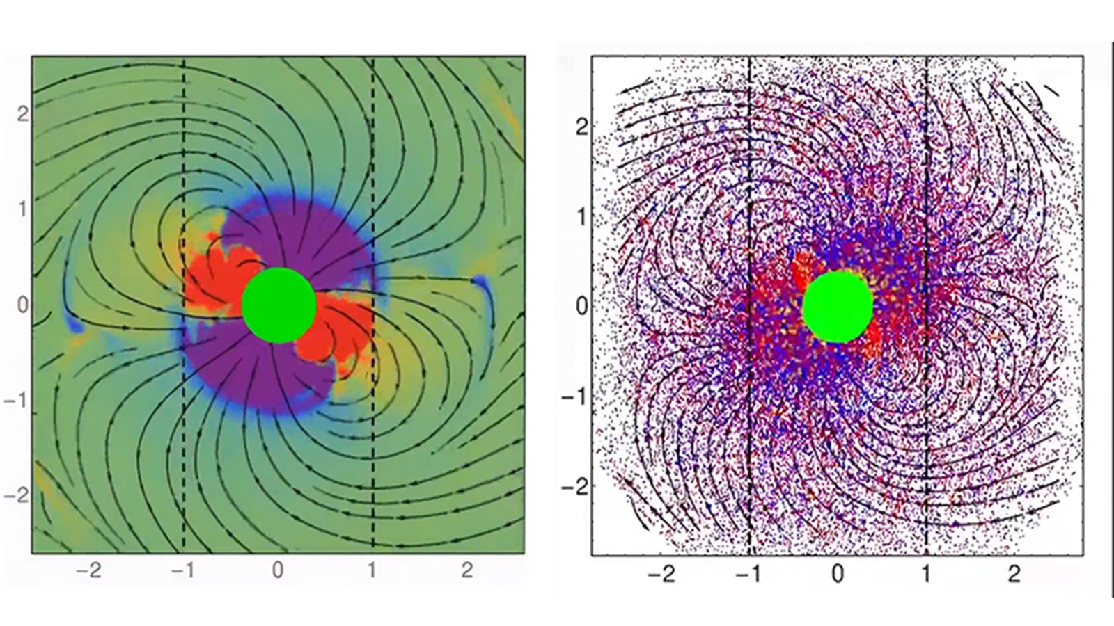
This video shows the evolution of a rotating pulsar's magnetosphere with a 45-degree magnetic inclination.
This video shows the evolution of a rotating pulsar's magnetosphere with a 45-degree magnetic inclination, from particle-in-cell simulations. The force-free (FF) solution forms as the equatorial current sheet emerges at the light-cylinder (dashed lines). The right panel shows field lines and particles (blue: electrons, red: positrons, yellow: new particles), while the left panel shows charge density, revealing the required charge excess matches the FF requirements despite electrons and positrons being everywhere.

Read More Constantinos Kalapotharakos, NASA/Goddard

Filter